This tutorial is part of a series on Simultaneous Localization and Mapping (SLAM) using the extended Kalman filter. See the following for other tutorials in the series:

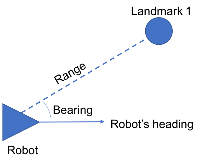
In this tutorial I’ll focus on one of the easiest state estimation problems: localization with known measurement correspondence. The “localization” part means that the robot already knows the positions of all of the landmarks in the environment. The “known correspondence” part means that when the robot measures the range and bearing to a landmark it always knows which landmark it’s measuring.

In this tutorial I’ll explain the EKF algorithm and then demonstrate how it can be implemented using the UTIAS dataset. I’ll break it down into the following sections:

Intro to the Algorithm
- Inputs
- Outputs
The Algorithm
- Motion Update
- Sensor Update
MATLAB code

Intro To The Algorithm

First off, why do we need this complicated algorithm for localization? Can’t we just track our position with odometry? This isn’t possible because a robot’s pose over time is not deterministic; it can’t be calculated exactly due to errors (also referred to as noise) in the odometry which accumulate over time.

This is why the Kalman filter represents the robot’s pose at time $t$ as a multivariate normal probability distribution with a mean at $\mu_t$ and covariance of $\Sigma_t$ . The robot’s expected (or most likely) pose is at $\mu_t$ and the uncertainty of that pose is quantified by $\Sigma_t$ . The Kalman filter updates the robot’s pose using the robot’s motion from odometry $u_t$ . Then it corrects for noise in the motion update using the robot’s sensor readings $z_t$ .

One important advantage of the Kalman filter (and other similar algorithms) is that it is recursive. It only requires information about the state of the robot at time $t-1$ in order to estimate the state at time $t$ . In other words, it doesn’t require information about any of the prior states of the robot from time $t_0$ to time $t-2$ . This means it requires less memory and processor time to compute!

Below I present a mathematical definition for the extended Kalman filter. Most of it is taken from table 7.2 of Probabilistic Robotics by Thrun, Fox, and Burgard. It will be helpful to follow along in Probabilistic Robotics in addition to this tutorial. I’d also recommend reading chapter 3 of that book to gain a better understanding of Gaussian filters and recursive estimation.

Top of page

Inputs

the mean of the pose estimate from the previous timestep:
- $x_{t-1}$ is the robot’s previous x position in meters
- $y_{t-1}$ is the robot’s previous y position in meters
- $\theta_{t-1}$ is the robot’s previous heading in radians
the covariance matrix of the previous timestep,
- this represents the uncertainty of the pose estimate
the control inputs (or odometry) at the current timestep,
- $v_t$ is the robot’s linear velocity in meters/sec
- $\omega_t$ is the robot’s angular velocity in radians/sec
the measurements from the current timestep, where is the number of measurements at time
- each where
  - $r_t^i$ is the range to landmark $i$ in meters
  - $\phi_t^i$ is the bearing to landmark $i$ in radians
  - $s_t^i$ is the ID of landmark $i$
is the correspondence between the measurement and landmarks
- for our purposes this will be ignored for now
the map where is the number of landmarks
- each where
  - $m_{i,x}$ is the x position of landmark $i$ in meters
  - $m_{i,y}$ is the y position of landmark $i$ in meters
  - $m_{i,s}$ is the ID of landmark $i$

Top of page

Outputs

the updated pose estimate, $\mu_t$
the updated covariance matrix, $\Sigma_t$
the measurement probability, , which is the likelihood of the measurements given the robot’s estimated pose before measurements were incorporated:
- We’ll be ignoring this for now as well

Top of page

Algorithm

$\begin{flalign*} \text{Loc} &\text{alization with known correspondence}(\mu_{t-1}, \Sigma_{t-1},u_t,z_t,c_t,m): \\ &\theta = u_{t-1,\theta} \\ &G_t = \begin{bmatrix} 1 &0 &-v_t \Delta t \sin(\theta + \frac{\omega_t \Delta t}{2})\\ 0 &1 &v_t \Delta t \cos(\theta + \frac{\omega_t \Delta t}{2})\\ 0 &0 &1 \end{bmatrix} \\ &V_t = \begin{bmatrix} \cos(\theta + \frac{\omega_t \Delta t}{2}) &-\frac{1}{2} \sin(\theta + \frac{\omega_t \Delta t}{2}) \\ \sin(\theta + \frac{\omega_t \Delta t}{2}) &\frac{1}{2} \cos(\theta + \frac{\omega_t \Delta t}{2}) \\ 0 &1 \end{bmatrix} \\ &M_t = \begin{bmatrix} \alpha_1 v_{t}^{2} + \alpha_2 \omega_{t}^{2} &0 \\ 0 &\alpha_{3} v_{t}^{2} + \alpha_4 \omega_{t}^{2} \end{bmatrix} \\ &\bar{\mu_t} = \mu_{t-1} + \begin{bmatrix} v_t \Delta t \cos(\theta + \frac{\omega_t \Delta t}{2}) \\ v_t \Delta t \sin(\theta + \frac{\omega_t \Delta t}{2}) \\ \omega_t \Delta t \end{bmatrix} \\ &\bar{\Sigma}_t = G_t \Sigma_{t-1} G_{t}^{T} + V_t M_t V_{t}^{T} \\ &Q_t = \begin{bmatrix} \sigma_{r}^{2} &0 &0 \\ 0 &\sigma_{\phi}^{2} &0 \\ 0 &0 &\sigma_{s}^{2} \end{bmatrix}\\ &\text{for all observed features $z_{t}^{i}=\begin{bmatrix} r_{t}^{i} &\phi_{t}^{i} &s_{t}^{i}\end{bmatrix}^T$ do} \\ \end{flalign*}$

$\begin{flalign*} &j=c_{t}^{i}\\ &q = (m_{j,x} - \bar{\mu}_{t,x})^2 + (m_{j,y} - \bar{\mu}_{t,y})^2 \\ &\hat{z}_{t}^{i} = \begin{bmatrix} \sqrt{q} \\ \text{atan2}(m_{j,y} - \bar{\mu}_{t,y} \text{, }m_{j,x} - \bar{\mu}_{t,x}) - \bar{\mu}_{t, \theta} \\ m_{j,s} \end{bmatrix} \\ &H_{t}^{i} = \begin{bmatrix} -\frac{m_{j,x} - \bar{\mu}_{t,x}}{\sqrt{q}} & -\frac{m_{j,y} - \bar{\mu}_{t,y}}{\sqrt{q}} &0 \\ \frac{m_{j,y} - \bar{\mu}_{t,y}}{q} &-\frac{m_{j,x} - \bar{\mu}_{t,x}}{q} &-1 \\ 0 &0 &0 \end{bmatrix} \\ &S_{t}^{i} = H_{t}^{i} \bar{\Sigma}_t \lbrack H_{t}^{i} \rbrack ^T + Q_t \\ &K_{t}^{i} = \bar{\Sigma}_t \lbrack H_{t}^{i} \rbrack ^T \lbrack S_{t}^{i} \rbrack ^{-1} \\ &\bar{\mu}_t = \bar{\mu}_t + K_{t}^{i}(z_{t}^{i} - \hat{z}_{t}^{i}) \\ &\bar{\Sigma}_t = (I - K_{t}^{i} H_t^i) \bar{\Sigma}_t \\ \end{flalign*}$

$\begin{flalign*} &\text{end for} \\ &\mu_t = \bar{\mu}_t \\ &\Sigma_t = \bar{\Sigma}_t \\ &p_{z_t} = \prod_i \det(2 \pi S_t^i)^{-\frac{1}{2}} \exp \{ -\frac{1}{2}(z_t^i - \hat{z}_t^i)^T \lbrack S_t^i \rbrack ^{-1} (z_t^i - \hat{z}_t^i) \} \\ &\text{return } \mu_t, \Sigma_t, p_{z_t} \\ \end{flalign*}$

Top of page

Motion Update

The algorithm is divided into two parts: the motion update and the sensor update. First, in the motion update the odometry information is incorporated into the state estimate. The motion update is based around a motion model $g(u_t, x_{t-1})$ , which calculates a new pose based on the previous pose $x_{t-1}$ and the odometry $u_t$ .

(1) $\begin{equation*} \bar{\mu_t} = g(u_t, x_{t-1}) = \mu_{t-1} + \begin{bmatrix} v_t \Delta t \cos(\theta + \frac{\omega_t \Delta t}{2}) \\ v_t \Delta t \sin(\theta + \frac{\omega_t \Delta t}{2}) \\ \omega_t \Delta t \end{bmatrix} \end{equation*}$

In this equation $\bar{\mu}_t$ denotes the estimated updated mean of the pose distribution. The motion model I’m using assumes that the robot rotates in place, then drives in a straight line, then rotates in place again. This is a common approximation and it’s accurate enough as long as $\Delta t$ is small.

In addition to calculating a new mean for our robot’s pose distribution $\bar{\mu}_t$ we need calculate an estimated covariance for the new pose, $\bar{\Sigma}_t$ . In order to do this we need to multiply the covariance from the last timestep, $\Sigma_{t-1}$ by the derivative (also called the Jacobian) of the motion model with respect to the previous state $x_{t-1}$ :

(2) $\begin{equation*} G_t = \frac{\partial g(u_t, \mu_{t-1})}{\partial x_{t-1}} = \begin{bmatrix} 1 &0 &-v_t \Delta t \sin(\theta + \frac{\omega_t \Delta t}{2})\\ 0 &1 &v_t \Delta t \cos(\theta + \frac{\omega_t \Delta t}{2})\\ 0 &0 &1 \end{bmatrix} \end{equation*}$

The multiplication looks like the following: $G_t \Sigma_{t-1} G_t^T$ . We also need to calculate the additional noise (or uncertainty) associated with the motion that occurred between $t-1$ and $t$ .

(3) $\begin{equation*} M_t = \begin{bmatrix} \alpha_1 v_{t}^{2} + \alpha_2 \omega_{t}^{2} &0 \\ 0 &\alpha_{3} v_{t}^{2} + \alpha_4 \omega_{t}^{2} \end{bmatrix} \end{equation*}$

The alphas $\alpha_1$ through $\alpha_4$ are noise parameters that, unfortunately, need to be hand-tuned for the particular robot being used. Also, $M_t$ is in control space and we need to map it into state space. To do this we need the Jacobian of the motion model with respect to the motion parameters $u_t$ :

(4) $\begin{equation*} V_t = \frac{\partial g(u_t, \mu_{t-1})}{\partial u_t} = \begin{bmatrix} \cos(\theta + \frac{\omega_t \Delta t}{2}) &-\frac{1}{2} \sin(\theta + \frac{\omega_t \Delta t}{2}) \\ \sin(\theta + \frac{\omega_t \Delta t}{2}) &\frac{1}{2} \cos(\theta + \frac{\omega_t \Delta t}{2}) \\ 0 &1 \end{bmatrix} \end{equation*}$

So we can map the noise $M_t$ to state space with the following multiplication: $V_t M_t V_t^T$ . To get the complete updated covariance $\bar{\Sigma}_t$ we add the transformed covariance from the previous timestep to the additional noise:

(5) $\begin{equation*} \bar{\Sigma}_t = G_t \Sigma_{t-1} G_{t}^{T} + V_t M_t V_{t}^{T} \end{equation*}$

So the motion update step updates the robot’s pose mean and covariance based on its odometry. You may have noticed, however, that the covariance only gets larger in this step. This means our uncertainty about the robot’s pose always grows when we incorporate odometry. We can decrease the uncertainty by incorporating sensor information, which is what we do in the next step.

Note: The motion model and associated Jacobians presented in the preceding section are different from those presented in Probabilistic Robotics. The model presented in Probabilistic Robotics assumes that the robot is always moving in an arc and its angular velocity, $\omega_t$ , is never zero. The Jacobians for this model involve dividing by $\omega_t$ . This means that the model breaks if $\omega_t$ is ever equal to zero. This is a problem for us because $\omega_t$ often is equal to zero in the UTIAS dataset. That is why I subbed in my own motion model.

Top of page

Sensor Update

The sensor update refines the robot’s pose estimate and decreases its uncertainty. This happens in the for loop of the algorithm. It is run for every measurement that occurs at timestep $t$ .

In the first step of the sensor update we calculate what the range and bearing to the landmark would have been if the estimated pose mean $\bar{\mu}_t$ were correct. This is called the expected measurement $\hat{z}_t$ and it is calculated using the measurement model $h_t(x_t,m)$ .

(6) $\begin{equation*} q = (m_{j,x} - \bar{\mu}_{t,x})^2 + (m_{j,y} - \bar{\mu}_{t,y})^2 \end{equation*}$

(7) $\begin{equation*} \hat{z}_{t}^{i} = h(x_t, m) = \begin{bmatrix} \sqrt{q} \\ \text{atan2}(m_{j,y} - \bar{\mu}_{t,y} \text{, }m_{j,x} - \bar{\mu}_{t,x}) - \bar{\mu}_{t, \theta} \\ m_{j,s} \end{bmatrix} \\ \end{equation*}$

Remember that $m_{j,x}$ , $m_{j,y}$ , and $m_{j,s}$ are the x position, y position, and ID of landmark $j$ , respectively.

We also need to calculate the additional noise associated with the measurement. To do this we need the Jacobian of the measurement model with respect to the robot’s pose:

(8) $\begin{equation*} H_{t}^{i} = \frac{\partial h(\bar{\mu}_t, m)}{\partial x_t} = \begin{bmatrix} -\frac{m_{j,x} - \bar{\mu}_{t,x}}{\sqrt{q}} & -\frac{m_{j,y} - \bar{\mu}_{t,y}}{\sqrt{q}} &0 \\ \frac{m_{j,y} - \bar{\mu}_{t,y}}{q} &-\frac{m_{j,x} - \bar{\mu}_{t,x}}{q} &-1 \\ 0 &0 &0 \end{bmatrix} \end{equation*}$

The measurement noise is calculated by multiplying the prior estimated covariance with the measurement model Jacobian and adding additional noise for the new measurement. The additional noise $Q_t$ is a constant for all measurements. It is a $3 \times 3$ diagonal matrix with noise parameters $\sigma_r$ , $\sigma_\phi$ , and $\sigma_s$ . The sigmas represent the noise for landmark range, bearing, and noise, respectively. Like the alphas in equation (3), the sigmas must be hand-tuned in order to obtain good performance.

(9) $\begin{equation*} S_t^i = H_t^i \bar{\Sigma}_t \lbrack H_t^i \rbrack ^T + Q_t \end{equation*}$

$S_t^i$ is then used to calculate the Kalman gain, $K_t^i$ . The Kalman gain determines how heavily the sensor information should be weighted when correcting the estimated new pose $\bar{\mu}_t$ and $\bar{\Sigma}_t$ .

(10) $\begin{equation*} K_{t}^{i} = \bar{\Sigma}_t \lbrack H_{t}^{i} \rbrack ^T \lbrack S_{t}^{i} \rbrack ^{-1} \end{equation*}$

The Kalman gain is used to update the estimated pose mean and covariance $\bar{\mu}_t$ and $\bar{\Sigma}_t$ as follows:

(11) $\begin{equation*} \bar{\mu}_t = \bar{\mu}_t + K_{t}^{i}(z_{t}^{i} - \hat{z}_{t}^{i}) \end{equation*}$

(12) $\begin{equation*} \bar{\Sigma}_t = (I - K_{t}^{i} H_t^i) \bar{\Sigma}_t \end{equation*}$

The amount of correction to the estimated pose mean depends on $K_t^i$ and the difference between the expected measurement $\hat{z}_t^i$ (calculated in equation (7) and the actual measurement $z_t^i$ . A larger discrepancy between the expected and actual measurement will result in a larger correction.

After the sensor update is complete the pose mean and covariance are updated with the estimated values: $\mu_t = \bar{\mu}_t$ and $\Sigma_t = \bar{\Sigma}_t$ . The measurement probability is also calculated here but we are not making use of this value.

Top of page

Code

When writing robotics software I’m often frustrated by the separation between theory and software engineering. There are many good theoretical explanations of the extended Kalman filter online. There are also several good examples of code that uses an EKF. But I was unable to find any textbook, academic paper, blog post, or stackexchange thread that did a good job of demonstrating how the math translates into code. I’m hoping my code below will change that. I’ve been careful to explain all major steps and refer to the equations above in the comments. I hope you find it helpful!

Lastly, note that comments in MATLAB begin with a % symbol. The code rendering plugin I used doesn’t seem to get this when highlighting the code, however. So be aware that the highlighting below isn’t always accurate, but the actual code is.

addpath ../common; % adds support functions used in all my EKF programs
                   % check my github for details

deltaT = .02; 
alphas = [.2 .03 .09 .08 0 0]; % robot-dependent motion noise parameters
                               % see equation 3

% robot-dependent sensor noise parameters
% see equation 9
sigma_range = 2;
sigma_bearing = 3;
sigma_id = 1;

Q_t = [sigma_range^2 0 0;
       0 sigma_bearing^2 0;
       0 0 sigma_id^2];

measurement_prob = 0;
n_robots = 1;
robot_num = 1;

% load and resample raw data from UTIAS data set
% The robot's position groundtruth, odometry, and measurements 
% are stored in Robots
[Barcodes, Landmark_Groundtruth, Robots] = loadMRCLAMdataSet(n_robots);
[Robots, timesteps] = sampleMRCLAMdataSet(Robots, deltaT);

% add pose estimate matrix to Robots
% data will be added to this as the program runs
Robots{robot_num}.Est = zeros(size(Robots{robot_num}.G,1), 4);

% initialize time, and pose estimate
start = 600; % start index is set to 600 because earlier data was 
             % found to cause problems
t = Robots{robot_num}.G(start, 1); % set start time

% set starting pose mean to pose groundtruth at start time
poseMean = [Robots{robot_num}.G(start,2);
            Robots{robot_num}.G(start,3);
            Robots{robot_num}.G(start,4)];
poseCov = [0.01 0.01 0.01;
           0.01 0.01 0.01;
           0.01 0.01 0.01];
       
% tracks which measurement is next received
measurementIndex = 1;

% set up map between barcodes and landmark IDs
codeDict = containers.Map(Barcodes(:,2),Barcodes(:,1));

% advance measurement index until the next measurement time 
% is greater than the starting time
while (Robots{robot_num}.M(measurementIndex, 1) < t - .05)
        measurementIndex = measurementIndex + 1;
end

% loop through all odometry and measurement samples
% updating the robot's pose estimate with each step
% reference table 7.2 in Probabilistic Robotics
for i = start:size(Robots{robot_num}.G, 1)
    theta = poseMean(3, 1);
    % update time
    t = Robots{robot_num}.G(i, 1);
    % update movement vector per equation 1
    u_t = [Robots{robot_num}.O(i, 2); Robots{robot_num}.O(i, 3)];

    rot = deltaT * u_t(2);
    halfRot = rot / 2;
    trans = u_t(1) * deltaT;
    
    % calculate the movement Jacobian per equation 2
    G_t = [1 0 trans * -sin(theta + halfRot);
           0 1 trans * cos(theta + halfRot);
           0 0 1];
    % calculate motion covariance in control space per equation 3
    M_t = [(alphas(1) * abs(u_t(1)) + alphas(2) * abs(u_t(2)))^2 0;
           0 (alphas(3) * abs(u_t(1)) + alphas(4) * abs(u_t(2)))^2];
       
    % calculate Jacobian to transform motion covariance to state space
    % per equation 4
    V_t = [cos(theta + halfRot) -0.5 * sin(theta + halfRot);
           sin(theta + halfRot) 0.5 * cos(theta + halfRot);
           0 1];
    
    % calculate pose update
    poseUpdate = [trans * cos(theta + halfRot);
                  trans * sin(theta + halfRot);
                  rot];
              
    % calculate estimated pose mean per equation 1
    poseMeanBar = poseMean + poseUpdate;
    % calculate estimated pose covariance per equation 5
    poseCovBar = G_t * poseCov * G_t' + V_t * M_t * V_t';
    
    
    % get measurements for the current timestep, if any exist
    [z, measurementIndex] = getObservations(Robots, robot_num, t, measurementIndex, codeDict);
    
    % create two matrices for expected measurement and measurement
    % covariance
    S = zeros(size(z,2),3,3);
    zHat = zeros(3, size(z,2));
    
    % if any measurements are available
    if z(3,1) > 1
        for k = 1:size(z, 2) % loop over every measurement
            j = z(3,k);

            % get coordinates of the measured landmark
            m = Landmark_Groundtruth(j, 2:3);

            % compute the expected measurement per equations 6 and 7
            xDist = m(1) - poseMeanBar(1);
            yDist = m(2) - poseMeanBar(2);
            q = xDist^2 + yDist^2;
            
            % constrains expected bearing to between 0 and 2*pi
            pred_bear = conBear(atan2(yDist, xDist) - poseMeanBar(3));
            
            zHat(:,k) = [sqrt(q);
                         pred_bear;
                         j];

            % calculate Jacobian of the measurement model per equation 8
            H = [(-1 * (xDist / sqrt(q))) (-1 * (yDist / sqrt(q))) 0;
                 (yDist / q) (-1 * (xDist / q)) -1;
                 0 0 0];
             
            % compute S per equation 9
            S(k,:,:) = H * poseCovBar * H' + Q_t;

            % compute Kalman gain per equation 10
            K = poseCov * H' * inv(squeeze(S(k,:,:)));
                
            % update pose mean and covariance estimates
            % per equations 11 and 12
            poseMeanBar = poseMeanBar + K * (z(:,k) - zHat(:,k));
            poseCovBar = (eye(3) - (K * H)) * poseCovBar;
        end
    end
    
    % update pose mean and covariance
    % constrains heading to between 0 and 2*pi
    poseMean = poseMeanBar;
    poseMean(3) = conBear(poseMean(3));
    poseCov = poseCovBar;
    
    % add pose mean to estimated position vector
    Robots{robot_num}.Est(i,:) = [t poseMean(1) poseMean(2) poseMean(3)];
    
    % calculate error between mean pose and groundtruth
    % for testing only
    %{
    groundtruth = [Robots{robot_num}.G(i, 2); 
                   Robots{robot_num}.G(i, 3); 
                   Robots{robot_num}.G(i, 4)];
    error = groundtruth - poseMean;
    %}
   
end

% display results!
animateMRCLAMdataSet(Robots, Landmark_Groundtruth, timesteps, deltaT);

Note: My tuning of the noise parameters in the code below is workable. But I didn’t spend as much time on them as I did for subsequent iterations of this tutorial. If you’d like to play with them I’m sure you can improve on my tunings!

Top of page

Bot Blog

building my robot army one sketch at a time

Intro to the EKF Step 1: Localization With Known Correlation

Intro To The Algorithm

Inputs

Outputs

Algorithm

Motion Update

Sensor Update

Code