Intro to the EKF Step 2: Localization With Unknown Correspondence

This tutorial is part of a series on Simultaneous Localization and Mapping (SLAM) using the extended Kalman filter. See the following for other tutorials in the series:

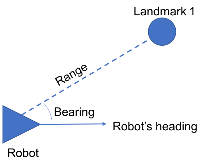
This tutorial will build incrementally on the previous tutorial: Localization With Known Correlation. We’re still just doing localization, which means the robot starts with a map of landmarks that does not change over the course of its run. The difference is this time when the robot gets a range and bearing measurement, it will not know to which landmark that measurement corresponds.

In this tutorial I will explain the process for estimating the correspondence between measurements and landmarks and present the correspondence algorithm on its own. Then I will show how the correspondence estimation algorithm can be integrated with the EKF localization algorithm introduced in the prior tutorial. As before, we’ll be using the UTIAS dataset for demonstration purposes.


Measurement Correspondence Intro

When our robot gets a measurement to a nearby landmark it can use that information to refine its estimate of its pose. In the last tutorial, each measurement received by our robot was in the form of z_t^i = [r_t^i\ \phi_t^i\ s_t^i]^T where z_t^i is the measurement to landmark i at time t. This vector contains the range r_t^i, bearing \phi_t^i, and, crucially, identity of the landmark being measured s_t^i. This could be interpreted as “landmark s is r meters away, at a bearing of \phi radians.”

In our current problem, the measurement vector will be z_t^i=[r_t^i\ \phi_t^i]^T. So we are no longer directly telling the robot to which landmark each measurement corresponds. Without knowledge of this correspondence measurements are basically useless to our robot. Sure, it knows the location of a landmark relative to its own location. But without knowing where that landmark is in the world it can’t use that information to refine its estimate of its pose.

So our robot needs a way to estimate the correspondence between its measurements and the landmarks in its map. One way it can do this is through maximum likelihood data association.


Maximum Likelihood Data Association

In maximum likelihood data association, as presented in section 7.5.2 of Probabilistic Robotics, the robot computes the probability that its current measurement corresponds to every landmark in its map. It then chooses the landmark with the highest probability of correspondence and assumes it is the correct association. This can be written as

\hat{c}_t = \text{argmax}_c\ p(z_t|c_{1:t},\ m,\ z_{1:t-1},\ u_{1:t})

In other words, given the robot’s past measurement correspondences c_{1:t}, map m, past measurements z_{1:t-1}, and past control inputs u_{1:t}, which landmark has the highest probability of producing measurement z_t?

In practice we find this by calculating the expected measurement and measurement covariance for every landmark in the map. We can then use these to calculate the measurement probability for every landmark and then select the landmark with the highest probability. The algorithm goes as follows:

    \begin{align*} \text{for all}&\text{ measurements } z_t^i=[r_t^i\ \phi_t^i]^T \text{ do} \\ \text{for}&\text{ all landmarks } k \text{ in the map } m \text{ do} \\ &q = (m_{k,x} - \bar{\mu}_{t,x})^2 + (m_{k,y} - \bar{\mu}_{t,y})^2 \\ &\hat{z}_t^k = \begin{bmatrix} \sqrt{q} \\ \text{atan2}(m_{k,y}-\bar{\mu}_{t,y},\ m_{k,x}-\bar{\mu}_{t,x})-\bar{\mu}_{t,\theta} \end{bmatrix} \\ &H_t^k = \begin{bmatrix} -\frac{m_{k,x}-\bar{\mu}_{t,x}}{\sqrt{q}} & -\frac{m_{k,y}-\bar{\mu}_{t,y}}{\sqrt{q}} & 0 \\ \frac{m_{k,y}-\bar{\mu}_{t,y}}{q} & -\frac{m_{k,x}-\bar{\mu}_{t,x}}{q} & -1\end{bmatrix} \\ &S_t^k = H_t^k \bar{\Sigma}_t [H_t^k]^T + Q_t \\ \text{end}&\text{for} \\ j(i) &= \text{argmax}_k\ \text{det}(2\pi S_t^k)^{-\frac{1}{2}} \text{exp}\{-\frac{1}{2}(z_t^i-\hat{z}_t^k)[S_t^k]^{-1}(z_t^i-\hat{z}_t^k)^T\}\\ \text{endfor}& \end{align*}

The end result j(i) is the estimated correspondence j for each measurement i. It should be noted that the probability estimates are conditioned on past correspondences. However, this method assumes that the past estimates are correct. This means that the correspondence estimates are very sensitive to incorrect associations; incorrect estimates are likely to remain incorrect on subsequent measurements. This makes the maximum likelihood method brittle and likely to diverge when measurements are incorrectly associated.

There are alternative methods that are more robust to incorrect associations. Multi-Hypothesis Tracking is one of these, but the maximum likelihood method is the simplest. For an introduction I think the maximum likelihood method is sufficient.


The Complete Algorithm

The code for the complete algorithm is shown below. It is the same as the code for EKF localization with known correlation with the addition of the maximum likelihood algorithm for measurement correspondence (lines 85 to 120). Note also that the code rendering program I’m using doesn’t seem to handle MATLAB code very well, and some of the highlighting is a little messed up.

addpath ../common;

deltaT = .02;
alphas = [.2 .03 .09 .08 0 0]; % motion model noise parameters

% measurement model noise parameters
sigma_range = .43;
sigma_bearing = .6;

Q_t = [sigma_range^2 0;
       0 sigma_bearing^2];

n_robots = 1;
robot_num = 1;
n_landmarks = 15;
[Barcodes, Landmark_Groundtruth, Robots] = loadMRCLAMdataSet(n_robots);
[Robots, timesteps] = sampleMRCLAMdataSet(Robots, deltaT);

% add pose estimate matrix to Robots
Robots{robot_num}.Est = zeros(size(Robots{robot_num}.G,1), 4);

start = 1; 
t = Robots{robot_num}.G(start, 1); 
% need mean and covariance for the initial pose estimate
poseMean = [Robots{robot_num}.G(start,2);
            Robots{robot_num}.G(start,3);
            Robots{robot_num}.G(start,4)];
poseCov = 0.01*eye(3);
       
measurementIndex = 1;

% set up map between barcodes and landmark IDs
codeDict = containers.Map(Barcodes(:,2),Barcodes(:,1));

while (Robots{robot_num}.M(measurementIndex, 1) < t - .05)
        measurementIndex = measurementIndex + 1;
end

% loop through all odometry and measurement samples
% updating the robot's pose estimate with each step
% reference table 7.3 in Probabilistic Robotics
for i = start:size(Robots{robot_num}.G, 1)
    theta = poseMean(3, 1);
    % update time
    t = Robots{robot_num}.G(i, 1);
    % update movement vector
    u_t = [Robots{robot_num}.O(i, 2); Robots{robot_num}.O(i, 3)];

    rot = deltaT * u_t(2);
    halfRot = rot / 2;
    trans = u_t(1) * deltaT;
    
    % calculate the movement Jacobian
    G_t = [1 0 trans * -sin(theta + halfRot);
           0 1 trans * cos(theta + halfRot);
           0 0 1];
    % calculate motion covariance in control space
    M_t = [(alphas(1) * abs(u_t(1)) + alphas(2) * abs(u_t(2)))^2 0;
           0 (alphas(3) * abs(u_t(1)) + alphas(4) * abs(u_t(2)))^2];
    % calculate Jacobian to transform motion covariance to state space
    V_t = [cos(theta + halfRot) -0.5 * sin(theta + halfRot);
           sin(theta + halfRot) 0.5 * cos(theta + halfRot);
           0 1];
    
    % calculate pose update from odometry
    poseUpdate = [trans * cos(theta + halfRot);
                  trans * sin(theta + halfRot);
                  rot];
    
    poseMeanBar = poseMean + poseUpdate;
    poseCovBar = G_t * poseCov * G_t' + V_t * M_t * V_t';
    
    % get measurements
    [z, measurementIndex] = getObservations(Robots, robot_num, t, measurementIndex, codeDict);
    
    % remove landmark ID from measurement because
    % we're trying to live without that
    z = z(1:2,:);
    
    % if features are observed
    % loop over all features and compute Kalman gain
    if z(1,1) > 0.1
        for k = 1:size(z, 2) % loop over every observed landmark
            
            % loop over all landmarks and compute MLE correspondence
            predZ = zeros(n_landmarks, 1, 2); % predicted measurements
            predS = zeros(n_landmarks, 2, 2); % predicted measurement covariances
            predH = zeros(n_landmarks, 2, 3); % predicted measurement Jacobians
            maxJ = 0; 
            landmarkIndex = 0;
            for j = 1:n_landmarks
                xDist = Landmark_Groundtruth(j, 2) - poseMeanBar(1);
                yDist = Landmark_Groundtruth(j, 3) - poseMeanBar(2);
                q = xDist^2 + yDist^2;
                
                % calculate predicted measurement
                predZ(j,:,:) = [sqrt(q);
                            conBear(atan2(yDist, xDist) - poseMeanBar(3))];
                        
                % calculate predicted measurement Jacobian
                predH(j,:,:) = [-xDist/sqrt(q) -yDist/sqrt(q) 0;
                                yDist/q        -xDist/q      -1];
                            
                % calculate predicted measurement covariance
                predS(j,:,:) = squeeze(predH(j,:,:)) * poseCovBar ...
                               * squeeze(predH(j,:,:))' + Q_t;
                
                % calculate probability of measurement correspondence          
                thisJ = det(2 * pi * squeeze(predS(j,:,:)))^(-0.5) * ...
                        exp(-0.5 * (z(:,k) - squeeze(predZ(j,:,:)))' ...
                        * inv(squeeze(predS(j,:,:))) ...
                        * (z(:,k) - squeeze(predZ(j,:,:))));
                
                % update correspondence if the probability is
                % higher than the previous maximum
                if thisJ > maxJ
                    maxJ = thisJ;
                    landmarkIndex = j;
                end
            end

            % compute Kalman gain
            K = poseCovBar * squeeze(predH(landmarkIndex,:,:))' ...
                * inv(squeeze(predS(landmarkIndex,:,:)));

            % update pose mean and covariance estimates
            poseMeanBar = poseMeanBar + K * (z(:,k) - squeeze(predZ(landmarkIndex,:,:)));
            poseCovBar = (eye(3) - (K * squeeze(predH(landmarkIndex,:,:)))) * poseCovBar;
        end
    end
    
    % update pose mean and covariance
    poseMean = poseMeanBar;
    poseMean(3) = conBear(poseMean(3));
    poseCov = poseCovBar;
    
    % add pose mean to estimated position vector
    Robots{robot_num}.Est(i,:) = [t poseMean(1) poseMean(2) poseMean(3)];
    
    % calculate error between mean pose and groundtruth 
    % for testing only
    %{
    groundtruth = [Robots{robot_num}.G(i, 2); 
                   Robots{robot_num}.G(i, 3); 
                   Robots{robot_num}.G(i, 4)];
    error = groundtruth - poseMean;
    %}
   
end
animateMRCLAMdataSet(Robots, Landmark_Groundtruth, timesteps, deltaT);

Intro to the EKF Step 1: Localization With Known Correlation

This tutorial is part of a series on Simultaneous Localization and Mapping (SLAM) using the extended Kalman filter. See the following for other tutorials in the series:

In this tutorial I’ll focus on one of the easiest state estimation problems: localization with known measurement correspondence. The “localization” part means that the robot already knows the positions of all of the landmarks in the environment. The “known correspondence” part means that when the robot measures the range and bearing to a landmark it always knows which landmark it’s measuring.

In this tutorial I’ll explain the EKF algorithm and then demonstrate how it can be implemented using the UTIAS dataset. I’ll break it down into the following sections:


Intro To The Algorithm

First off, why do we need this complicated algorithm for localization? Can’t we just track our position with odometry? This isn’t possible because a robot’s pose over time is not deterministic; it can’t be calculated exactly due to errors (also referred to as noise) in the odometry which accumulate over time.

This is why the Kalman filter represents the robot’s pose at time t as a multivariate normal probability distribution with a mean at \mu_t and covariance of \Sigma_t. The robot’s expected (or most likely) pose is at \mu_t and the uncertainty of that pose is quantified by \Sigma_t. The Kalman filter updates the robot’s pose using the robot’s motion from odometry u_t. Then it corrects for noise in the motion update using the robot’s sensor readings z_t.

One important advantage of the Kalman filter (and other similar algorithms) is that it is recursive. It only requires information about the state of the robot at time t-1 in order to estimate the state at time t. In other words, it doesn’t require information about any of the prior states of the robot from time t_0 to time t-2. This means it requires less memory and processor time to compute!

Below I present a mathematical definition for the extended Kalman filter. Most of it is taken from table 7.2 of Probabilistic Robotics by Thrun, Fox, and Burgard. It will be helpful to follow along in Probabilistic Robotics in addition to this tutorial. I’d also recommend reading chapter 3 of that book to gain a better understanding of Gaussian filters and recursive estimation.

Top of page


Inputs

  • the mean of the pose estimate from the previous timestep: \mu_{t-1} = \begin{bmatrix} x_{t-1} &y_{t-1} &\theta_{t-1} \end{bmatrix}^T
    • x_{t-1} is the robot’s previous x position in meters
    • y_{t-1} is the robot’s previous y position in meters
    • \theta_{t-1} is the robot’s previous heading in radians
  • the covariance matrix of the previous timestep, \Sigma_{t-1}
    • this represents the uncertainty of the pose estimate
  • the control inputs (or odometry) at the current timestep, u_t=\begin{bmatrix} v_t &\omega_t \end{bmatrix}^T
    • v_t is the robot’s linear velocity in meters/sec
    • \omega_t is the robot’s angular velocity in radians/sec
  • the measurements from the current timestep, z_t = \begin{bmatrix} z_t^1 &z_t^2 &\dots &z_t^k \end{bmatrix} where k is the number of measurements at time t
    • each z_t^i = \begin{bmatrix} r_t^i &\phi_t^i &s_t^i \end{bmatrix}^T where
      • r_t^i is the range to landmark i in meters
      • \phi_t^i is the bearing to landmark i in radians
      • s_t^i is the ID of landmark i
  • c_t is the correspondence between the measurement and landmarks
    • for our purposes this will be ignored for now
  • the map m = \begin{bmatrix}m_1 &m_2 &\dots &m_n \end{bmatrix} where n is the number of landmarks
    • each m_i = \begin{bmatrix} m_{i,x} &m_{i,y} &m_{i,s} \end{bmatrix}^T where
      • m_{i,x} is the x position of landmark i in meters
      • m_{i,y} is the y position of landmark i in meters
      • m_{i,s} is the ID of landmark i

Top of page


Outputs

  • the updated pose estimate, \mu_t
  • the updated covariance matrix, \Sigma_t
  • the measurement probability, p_{z_t}, which is the likelihood of the measurements z_t given the robot’s estimated pose before measurements were incorporated: \bar{\mu}_t
    • We’ll be ignoring this for now as well

Top of page


Algorithm

    \begin{flalign*} \text{Loc} &\text{alization with known correspondence}(\mu_{t-1}, \Sigma_{t-1},u_t,z_t,c_t,m): \\ &\theta = u_{t-1,\theta} \\ &G_t = \begin{bmatrix} 1 &0 &-v_t \Delta t \sin(\theta + \frac{\omega_t \Delta t}{2})\\ 0 &1 &v_t \Delta t \cos(\theta + \frac{\omega_t \Delta t}{2})\\ 0 &0 &1 \end{bmatrix} \\ &V_t = \begin{bmatrix} \cos(\theta + \frac{\omega_t \Delta t}{2}) &-\frac{1}{2} \sin(\theta + \frac{\omega_t \Delta t}{2}) \\ \sin(\theta + \frac{\omega_t \Delta t}{2}) &\frac{1}{2} \cos(\theta + \frac{\omega_t \Delta t}{2}) \\ 0 &1 \end{bmatrix} \\ &M_t = \begin{bmatrix} \alpha_1 v_{t}^{2} + \alpha_2 \omega_{t}^{2} &0 \\ 0 &\alpha_{3} v_{t}^{2} + \alpha_4 \omega_{t}^{2} \end{bmatrix} \\ &\bar{\mu_t} = \mu_{t-1} + \begin{bmatrix} v_t \Delta t \cos(\theta + \frac{\omega_t \Delta t}{2}) \\ v_t \Delta t \sin(\theta + \frac{\omega_t \Delta t}{2}) \\ \omega_t \Delta t \end{bmatrix} \\ &\bar{\Sigma}_t = G_t \Sigma_{t-1} G_{t}^{T} + V_t M_t V_{t}^{T} \\ &Q_t = \begin{bmatrix} \sigma_{r}^{2} &0 &0 \\ 0 &\sigma_{\phi}^{2} &0 \\ 0 &0 &\sigma_{s}^{2} \end{bmatrix}\\ &\text{for all observed features $z_{t}^{i}=\begin{bmatrix} r_{t}^{i} &\phi_{t}^{i} &s_{t}^{i}\end{bmatrix}^T$ do} \\ \end{flalign*}

    \begin{flalign*} &j=c_{t}^{i}\\ &q = (m_{j,x} - \bar{\mu}_{t,x})^2 + (m_{j,y} - \bar{\mu}_{t,y})^2 \\ &\hat{z}_{t}^{i} = \begin{bmatrix} \sqrt{q} \\ \text{atan2}(m_{j,y} - \bar{\mu}_{t,y} \text{,  }m_{j,x} - \bar{\mu}_{t,x}) - \bar{\mu}_{t, \theta} \\ m_{j,s} \end{bmatrix} \\ &H_{t}^{i} = \begin{bmatrix} -\frac{m_{j,x} - \bar{\mu}_{t,x}}{\sqrt{q}} & -\frac{m_{j,y} - \bar{\mu}_{t,y}}{\sqrt{q}} &0 \\ \frac{m_{j,y} - \bar{\mu}_{t,y}}{q} &-\frac{m_{j,x} - \bar{\mu}_{t,x}}{q} &-1 \\ 0 &0 &0 \end{bmatrix} \\ &S_{t}^{i} = H_{t}^{i} \bar{\Sigma}_t \lbrack H_{t}^{i} \rbrack ^T + Q_t \\ &K_{t}^{i} = \bar{\Sigma}_t \lbrack H_{t}^{i} \rbrack ^T \lbrack S_{t}^{i} \rbrack ^{-1} \\ &\bar{\mu}_t = \bar{\mu}_t + K_{t}^{i}(z_{t}^{i} - \hat{z}_{t}^{i}) \\ &\bar{\Sigma}_t = (I - K_{t}^{i} H_t^i) \bar{\Sigma}_t \\ \end{flalign*}

    \begin{flalign*} &\text{end for} \\ &\mu_t = \bar{\mu}_t \\ &\Sigma_t = \bar{\Sigma}_t \\ &p_{z_t} = \prod_i \det(2 \pi S_t^i)^{-\frac{1}{2}} \exp \{ -\frac{1}{2}(z_t^i - \hat{z}_t^i)^T \lbrack S_t^i \rbrack ^{-1} (z_t^i - \hat{z}_t^i) \} \\ &\text{return } \mu_t, \Sigma_t, p_{z_t} \\ \end{flalign*}

Top of page


Motion Update

The algorithm is divided into two parts: the motion update and the sensor update. First, in the motion update the odometry information is incorporated into the state estimate. The motion update is based around a motion model g(u_t, x_{t-1}), which calculates a new pose based on the previous pose x_{t-1} and the odometry u_t.

(1)   \begin{equation*} \bar{\mu_t} = g(u_t, x_{t-1}) = \mu_{t-1} + \begin{bmatrix} v_t \Delta t \cos(\theta + \frac{\omega_t \Delta t}{2}) \\ v_t \Delta t \sin(\theta + \frac{\omega_t \Delta t}{2}) \\ \omega_t \Delta t \end{bmatrix} \end{equation*}

In this equation \bar{\mu}_t denotes the estimated updated mean of the pose distribution. The motion model I’m using assumes that the robot rotates in place, then drives in a straight line, then rotates in place again. This is a common approximation and it’s accurate enough as long as \Delta t is small.

In addition to calculating a new mean for our robot’s pose distribution \bar{\mu}_t we need calculate an estimated covariance for the new pose, \bar{\Sigma}_t. In order to do this we need to multiply the covariance from the last timestep, \Sigma_{t-1}  by the derivative (also called the Jacobian) of the motion model with respect to the previous state x_{t-1}:

(2)   \begin{equation*} G_t = \frac{\partial g(u_t, \mu_{t-1})}{\partial x_{t-1}} = \begin{bmatrix} 1 &0 &-v_t \Delta t \sin(\theta + \frac{\omega_t \Delta t}{2})\\ 0 &1 &v_t \Delta t \cos(\theta + \frac{\omega_t \Delta t}{2})\\ 0 &0 &1 \end{bmatrix} \end{equation*}

The multiplication looks like the following: G_t \Sigma_{t-1} G_t^T. We also need to calculate the additional noise (or uncertainty) associated with the motion that occurred between t-1 and t.

(3)   \begin{equation*} M_t = \begin{bmatrix} \alpha_1 v_{t}^{2} + \alpha_2 \omega_{t}^{2} &0 \\ 0 &\alpha_{3} v_{t}^{2} + \alpha_4 \omega_{t}^{2} \end{bmatrix} \end{equation*}

The alphas \alpha_1 through \alpha_4 are noise parameters that, unfortunately, need to be hand-tuned for the particular robot being used. Also, M_t is in control space and we need to map it into state space. To do this we need the Jacobian of the motion model with respect to the motion parameters u_t:

(4)   \begin{equation*} V_t = \frac{\partial g(u_t, \mu_{t-1})}{\partial u_t} = \begin{bmatrix} \cos(\theta + \frac{\omega_t \Delta t}{2}) &-\frac{1}{2} \sin(\theta + \frac{\omega_t \Delta t}{2}) \\ \sin(\theta + \frac{\omega_t \Delta t}{2}) &\frac{1}{2} \cos(\theta + \frac{\omega_t \Delta t}{2}) \\ 0 &1 \end{bmatrix} \end{equation*}

So we can map the noise M_t to state space with the following multiplication: V_t M_t V_t^T. To get the complete updated covariance \bar{\Sigma}_t we add the transformed covariance from the previous timestep to the additional noise:

(5)   \begin{equation*} \bar{\Sigma}_t = G_t \Sigma_{t-1} G_{t}^{T} + V_t M_t V_{t}^{T} \end{equation*}

So the motion update step updates the robot’s pose mean and covariance based on its odometry. You may have noticed, however, that the covariance only gets larger in this step. This means our uncertainty about the robot’s pose always grows when we incorporate odometry. We can decrease the uncertainty by incorporating sensor information, which is what we do in the next step.

Note: The motion model and associated Jacobians presented in the preceding section are different from those presented in Probabilistic Robotics. The model presented in Probabilistic Robotics assumes that the robot is always moving in an arc and its angular velocity, \omega_t, is never zero. The Jacobians for this model involve dividing by \omega_t. This means that the model breaks if \omega_t is ever equal to zero. This is a problem for us because \omega_t often is equal to zero in the UTIAS dataset. That is why I subbed in my own motion model.

Top of page


Sensor Update

The sensor update refines the robot’s pose estimate and decreases its uncertainty. This happens in the for loop of the algorithm. It is run for every measurement that occurs at timestep t.

In the first step of the sensor update we calculate what the range and bearing to the landmark would have been if the estimated pose mean \bar{\mu}_t were correct. This is called the expected measurement \hat{z}_t and it is calculated using the measurement model h_t(x_t,m).

(6)   \begin{equation*} q = (m_{j,x} - \bar{\mu}_{t,x})^2 + (m_{j,y} - \bar{\mu}_{t,y})^2 \end{equation*}

(7)   \begin{equation*} \hat{z}_{t}^{i} = h(x_t, m) = \begin{bmatrix} \sqrt{q} \\ \text{atan2}(m_{j,y} - \bar{\mu}_{t,y} \text{,  }m_{j,x} - \bar{\mu}_{t,x}) - \bar{\mu}_{t, \theta} \\ m_{j,s} \end{bmatrix} \\ \end{equation*}

Remember that m_{j,x}, m_{j,y}, and m_{j,s} are the x position, y position, and ID of landmark j, respectively.

We also need to calculate the additional noise associated with the measurement. To do this we need the Jacobian of the measurement model with respect to the robot’s pose:

(8)   \begin{equation*} H_{t}^{i} = \frac{\partial h(\bar{\mu}_t, m)}{\partial x_t} = \begin{bmatrix} -\frac{m_{j,x} - \bar{\mu}_{t,x}}{\sqrt{q}} & -\frac{m_{j,y} - \bar{\mu}_{t,y}}{\sqrt{q}} &0 \\ \frac{m_{j,y} - \bar{\mu}_{t,y}}{q} &-\frac{m_{j,x} - \bar{\mu}_{t,x}}{q} &-1 \\ 0 &0 &0 \end{bmatrix} \end{equation*}

The measurement noise is calculated by multiplying the prior estimated covariance with the measurement model Jacobian and adding additional noise for the new measurement. The additional noise Q_t is a constant for all measurements. It is a 3 \times 3 diagonal matrix with noise parameters \sigma_r, \sigma_\phi, and \sigma_s. The sigmas represent the noise for landmark range, bearing, and noise, respectively. Like the alphas in equation (3), the sigmas must be hand-tuned in order to obtain good performance.

(9)   \begin{equation*} S_t^i = H_t^i \bar{\Sigma}_t \lbrack H_t^i \rbrack ^T + Q_t \end{equation*}

S_t^i is then used to calculate the Kalman gain, K_t^i. The Kalman gain determines how heavily the sensor information should be weighted when correcting the estimated new pose \bar{\mu}_t and \bar{\Sigma}_t.

(10)   \begin{equation*} K_{t}^{i} = \bar{\Sigma}_t \lbrack H_{t}^{i} \rbrack ^T \lbrack S_{t}^{i} \rbrack ^{-1} \end{equation*}

The Kalman gain is used to update the estimated pose mean and covariance \bar{\mu}_t and \bar{\Sigma}_t as follows:

(11)   \begin{equation*} \bar{\mu}_t = \bar{\mu}_t + K_{t}^{i}(z_{t}^{i} - \hat{z}_{t}^{i}) \end{equation*}

(12)   \begin{equation*} \bar{\Sigma}_t = (I - K_{t}^{i} H_t^i) \bar{\Sigma}_t \end{equation*}

The amount of correction to the estimated pose mean depends on K_t^i and the difference between the expected measurement \hat{z}_t^i (calculated in equation (7) and the actual measurement z_t^i. A larger discrepancy between the expected and actual measurement will result in a larger correction.

After the sensor update is complete the pose mean and covariance are updated with the estimated values: \mu_t = \bar{\mu}_t and \Sigma_t = \bar{\Sigma}_t. The measurement probability is also calculated here but we are not making use of this value.

Top of page


Code

When writing robotics software I’m often frustrated by the separation between theory and software engineering. There are many good theoretical explanations of the extended Kalman filter online. There are also several good examples of code that uses an EKF. But I was unable to find any textbook, academic paper, blog post, or stackexchange thread that did a good job of demonstrating how the math translates into code. I’m hoping my code below will change that. I’ve been careful to explain all major steps and refer to the equations above in the comments. I hope you find it helpful!

Lastly, note that comments in MATLAB begin with a % symbol. The code rendering plugin I used doesn’t seem to get this when highlighting the code, however. So be aware that the highlighting below isn’t always accurate, but the actual code is.

addpath ../common; % adds support functions used in all my EKF programs
                   % check my github for details

deltaT = .02; 
alphas = [.2 .03 .09 .08 0 0]; % robot-dependent motion noise parameters
                               % see equation 3

% robot-dependent sensor noise parameters
% see equation 9
sigma_range = 2;
sigma_bearing = 3;
sigma_id = 1;

Q_t = [sigma_range^2 0 0;
       0 sigma_bearing^2 0;
       0 0 sigma_id^2];

measurement_prob = 0;
n_robots = 1;
robot_num = 1;

% load and resample raw data from UTIAS data set
% The robot's position groundtruth, odometry, and measurements 
% are stored in Robots
[Barcodes, Landmark_Groundtruth, Robots] = loadMRCLAMdataSet(n_robots);
[Robots, timesteps] = sampleMRCLAMdataSet(Robots, deltaT);

% add pose estimate matrix to Robots
% data will be added to this as the program runs
Robots{robot_num}.Est = zeros(size(Robots{robot_num}.G,1), 4);

% initialize time, and pose estimate
start = 600; % start index is set to 600 because earlier data was 
             % found to cause problems
t = Robots{robot_num}.G(start, 1); % set start time

% set starting pose mean to pose groundtruth at start time
poseMean = [Robots{robot_num}.G(start,2);
            Robots{robot_num}.G(start,3);
            Robots{robot_num}.G(start,4)];
poseCov = [0.01 0.01 0.01;
           0.01 0.01 0.01;
           0.01 0.01 0.01];
       
% tracks which measurement is next received
measurementIndex = 1;

% set up map between barcodes and landmark IDs
codeDict = containers.Map(Barcodes(:,2),Barcodes(:,1));

% advance measurement index until the next measurement time 
% is greater than the starting time
while (Robots{robot_num}.M(measurementIndex, 1) < t - .05)
        measurementIndex = measurementIndex + 1;
end

% loop through all odometry and measurement samples
% updating the robot's pose estimate with each step
% reference table 7.2 in Probabilistic Robotics
for i = start:size(Robots{robot_num}.G, 1)
    theta = poseMean(3, 1);
    % update time
    t = Robots{robot_num}.G(i, 1);
    % update movement vector per equation 1
    u_t = [Robots{robot_num}.O(i, 2); Robots{robot_num}.O(i, 3)];

    rot = deltaT * u_t(2);
    halfRot = rot / 2;
    trans = u_t(1) * deltaT;
    
    % calculate the movement Jacobian per equation 2
    G_t = [1 0 trans * -sin(theta + halfRot);
           0 1 trans * cos(theta + halfRot);
           0 0 1];
    % calculate motion covariance in control space per equation 3
    M_t = [(alphas(1) * abs(u_t(1)) + alphas(2) * abs(u_t(2)))^2 0;
           0 (alphas(3) * abs(u_t(1)) + alphas(4) * abs(u_t(2)))^2];
       
    % calculate Jacobian to transform motion covariance to state space
    % per equation 4
    V_t = [cos(theta + halfRot) -0.5 * sin(theta + halfRot);
           sin(theta + halfRot) 0.5 * cos(theta + halfRot);
           0 1];
    
    % calculate pose update
    poseUpdate = [trans * cos(theta + halfRot);
                  trans * sin(theta + halfRot);
                  rot];
              
    % calculate estimated pose mean per equation 1
    poseMeanBar = poseMean + poseUpdate;
    % calculate estimated pose covariance per equation 5
    poseCovBar = G_t * poseCov * G_t' + V_t * M_t * V_t';
    
    
    % get measurements for the current timestep, if any exist
    [z, measurementIndex] = getObservations(Robots, robot_num, t, measurementIndex, codeDict);
    
    % create two matrices for expected measurement and measurement
    % covariance
    S = zeros(size(z,2),3,3);
    zHat = zeros(3, size(z,2));
    
    % if any measurements are available
    if z(3,1) > 1
        for k = 1:size(z, 2) % loop over every measurement
            j = z(3,k);

            % get coordinates of the measured landmark
            m = Landmark_Groundtruth(j, 2:3);

            % compute the expected measurement per equations 6 and 7
            xDist = m(1) - poseMeanBar(1);
            yDist = m(2) - poseMeanBar(2);
            q = xDist^2 + yDist^2;
            
            % constrains expected bearing to between 0 and 2*pi
            pred_bear = conBear(atan2(yDist, xDist) - poseMeanBar(3));
            
            zHat(:,k) = [sqrt(q);
                         pred_bear;
                         j];

            % calculate Jacobian of the measurement model per equation 8
            H = [(-1 * (xDist / sqrt(q))) (-1 * (yDist / sqrt(q))) 0;
                 (yDist / q) (-1 * (xDist / q)) -1;
                 0 0 0];
             
            % compute S per equation 9
            S(k,:,:) = H * poseCovBar * H' + Q_t;

            % compute Kalman gain per equation 10
            K = poseCov * H' * inv(squeeze(S(k,:,:)));
                
            % update pose mean and covariance estimates
            % per equations 11 and 12
            poseMeanBar = poseMeanBar + K * (z(:,k) - zHat(:,k));
            poseCovBar = (eye(3) - (K * H)) * poseCovBar;
        end
    end
    
    % update pose mean and covariance
    % constrains heading to between 0 and 2*pi
    poseMean = poseMeanBar;
    poseMean(3) = conBear(poseMean(3));
    poseCov = poseCovBar;
    
    % add pose mean to estimated position vector
    Robots{robot_num}.Est(i,:) = [t poseMean(1) poseMean(2) poseMean(3)];
    
    % calculate error between mean pose and groundtruth
    % for testing only
    %{
    groundtruth = [Robots{robot_num}.G(i, 2); 
                   Robots{robot_num}.G(i, 3); 
                   Robots{robot_num}.G(i, 4)];
    error = groundtruth - poseMean;
    %}
   
end

% display results!
animateMRCLAMdataSet(Robots, Landmark_Groundtruth, timesteps, deltaT);

Note: My tuning of the noise parameters in the code below is workable. But I didn’t spend as much time on them as I did for subsequent iterations of this tutorial. If you’d like to play with them I’m sure you can improve on my tunings!

Top of page

Intro to the EKF Step 0: The Data

This post is part of a series on SLAM with the extended Kalman filter. For other posts in the series see below.

Intro To The UTIAS Dataset

Writing programs for actual robots is difficult. Robots are expensive, testing code takes a lot of time, and the results are often difficult to interpret. This is why we don’t do most of our software development on actual robots. Instead it is much easier to run the actual robot once and log all of the robot’s sensor data, command inputs, and other relevant data. This way we can test our software on the logged data in a few seconds rather than doing a new test run every time we make a change to our code.

Setup used to make the UTIAS dataset

However, it’s difficult to make our own datasets for localization and mapping. In order to evaluate the accuracy of our SLAM software we need to know the actual (or groundtruth) pose of the robot with high accuracy at all times. This requires the use of motion capture setups which are well beyond the reach of most hobbyists. The good news is that university research groups routinely make their data sets available to the public. One such data set that is useful for our purposes is the UTIAS Multi-Robot Localization and Mapping (MRCLAM) dataset from the Autonomous Space Robotics Lab at the University of Toronto. I’ll refer to it as the UTIAS dataset for short.

The UTIAS data includes everything we’ll need to test our localization and mapping software: logs of the robot’s sensor data, accurate groundtruth poses for the robots throughout the run, and groundtruth positions for each landmark. I’ll go through each of those in detail below. You should take this opportunity download and extract “Dataset 1” from the download section of the MRCLAM webpage. You should also read the “Data Collection Details” of that page.


The Robots

The UTIAS dataset actually includes data from five different robots, all of which were run at the same time. This is because the dataset was originally intended for use in cooperative localization and mapping. However, this adds an unnecessary complication for our purposes. We will only be using the data from robot 1 in this tutorial.

The Measurements

The robot’s measurements are split up into two files: one for landmark measurements (Robot1_Measurements.dat) and one for odometry data (Robot1_Odometry.dat).

Illustration of a landmark measurement.

Each line of the Measurements file represents a measurement of a single landmark. We define a “measurement” with three quantities: range, the distance between the robot and the landmark in meters; bearing, the angle in radians between the landmark and the robot’s heading; and landmark ID, the unique identifier of the landmark being measured. Each line of the measurements file records the time the measurement occurred, the barcode for the landmark that was measured, the range, and the bearing. Note that the landmark barcode in the measurements file is not equivalent to the landmark ID in the landmark groundtruth file. The barcodes.dat file defines the mapping between the landmark barcodes and ID numbers.

The odometry file is pretty simple by comparison. Each line specifies the time, the robot’s linear velocity (in m/s), and its angular velocity (in rad/s).

The Groundtruth

Robot1_Groundtruth.dat specifies the robot’s actual pose in the global reference frame at any given time throughout the run. This is the part of the dataset that required the use of a motion capture system. Most of us could not recreate this on our own, so it’s nice that the University of Toronto made their data publicly available. Each line of the groundtruth file specifies the time, the robot’s x position in meters, the robot’s y position in meters, and the robot’s heading in radians.


The Landmarks

Landmark_Groundtruth.dat specifies the actual position of all of the landmarks in the environment. Each line specifies the landmark ID number, the x position, the y position, the standard deviation of the x position, and the std dev of the y position.


The Utilities

There are also a few useful MATLAB scripts available on the MRCLAM webpage.

loadMRCLAMdataSet.m will load the information in the .dat files into MATLAB variables. sampleMRCLAMdataSet.m will resample the data at 50Hz. This means that all of the measurements, odometry, and groundtruth information will come in at a predictable time interval. That will make things much easier. Lastly, animateMRCLAMdataSet.m will animate the motion of the robots throughout the run.

The problem with these scripts is they assume we want to work with all 5 robots. There are adapted versions of the scripts in my GitHub repo that only work with robot 1. Additionally, I adapted animateMRCLAMdataSet.m to animate both the groundtruth pose of robot 1 and the pose estimated by the EKF localization program. This will allow us to see just how well our program’s pose estimate tracks the robot’s true pose.

Intro to the Extended Kalman Filter

I started a PhD in computer science at CU Boulder four months ago. This is mainly because three years ago I made a wager. Since then I’ve become completely fascinated with robotics and have decided to pursue robotics research as a career.

Colin with his new sonar

Colin, my robot

I’m currently working at the ARPG at CU Boulder. As part of that work I wrote an implementation of SLAM using the Extended Kalman Filter (EKF). The EKF is the oldest probabilistic SLAM method. It’s a great introduction to SLAM techniques. However, it’s not very good by modern standards; it’s computationally expensive and it requires hand tuning several parameters to achieve passably accurate operation. But it is a good step in learning SLAM techniques, and I will likely implement an EKF on Colin at some point.

Tutorial Structure

Over the next several posts I’ll take you through my implementation of EKF SLAM in several steps. At the first step the robot will have a lot of prior knowledge about its environment and sensor readings. We’ll progressively take away pieces of the robot’s prior knowledge, making the task harder and harder as we go. In our last step the robot will have no prior knowledge. Our solution to this last step will be a fully-fledged SLAM program.

See the following for links to other tutorials in this series:

Dataset

I will use the UTIAS robot localization dataset for my tutorials. I’ll go into more detail on how to use and interpret the UTIAS data in my next post. The important thing to understand is that the UTIAS data abstracts away large parts of the SLAM problem such as controls and computer vision. This means we can just focus on programming and tuning our Extended Kalman Filters when using the UTIAS data. However, it also means we can’t simply upload our EKF programs to Colin. We would also need to write supporting programs that could supply data to the EKF in a form it can use.

Reference Material

Most of the math I’ll present in the next several posts came from Probabilistic Robotics, by Thrun, Fox, and Burgard. It’s a great book for anyone who wants to learn the theory behind fundamental robotics problems. It’s also not difficult to find a free pdf copy of an earlier edition if you don’t want to pay $85 for the current edition. But be warned that there are some math errors in the free pdf edition, so you may need to re-derive some things if you use it.

Probabilistic Robotics has a great section on Extended Kalman Filters and I’d recommend reading it thoroughly. However, the motion model it presents can’t be used with the UTIAS dataset so I’ll be using a different one. I’ll highlight where I deviate from the method presented in Probabilistic Robotics so as not to confuse those of you who are using it as a reference.

Programming Note

Lastly, the code I’m presenting is written in MATLAB. For those who don’t have access to MATLAB I would suggest using Python and NumPy. NumPy has all of the required functions to complete these tutorials. The only thing to watch out for is that Python uses zero-based indexing while MATLAB uses one-based indexing. If you don’t keep this in mind it could cause you some serious headaches.

I’m Learning Multithreading!

Since this quarter started I’ve been doing a weekly interview practice session with friends from school. Last week we spent most of our hour on this:

Rotate Matrix: Given an image represented by an NxN matrix, where each pixel in the image is 4 bytes, write a method to rotate the image by 90 degrees. Can you do this in place?

For those interested, it’s exercise 1.7 in the sixth edition of Cracking the Coding Interview by Gayle Laakmann McDowell. It’s a great interview prep book that’s been really helpful since I started job hunting. I had a lot of fun with this one so I’d like to do a short write up on our thought process.


Row-to-Column Method

The obvious thing to do here is create a new NxN square matrix and transpose the rows of the old matrix into the columns of the new matrix as in the graphic below:

MatrixRotateRtC

The above method takes O(n) time and O(n) space where n is the number of entries in the matrix. Coding this up should be pretty simple so I’m going to skip ahead to the thing I’m actually interested in: the in-place method.


In-Place Method

We can’t get below O(n) time to rotate a matrix since every entry must be moved and there are n entries. However, it is possible to cut the space usage down from O(n) to O(1) by doing the rotation in place. See the graphic below for an illustration of the method:

MatrixRotateIP

How do we implement this in code? It’s a little difficult but the key insight is that it’s possible to find the destination index for any given entry in the matrix from its starting index. In general terms the destination index can be found using this relation

Destination for { i, j } = { j, n – i }

where n is the last index in the matrix. The really cool thing about this is that it works for any starting index. The graphic above only shows a rotation of the outer layer of the matrix but the above method works for any index in any size of square matrix.

The code I post on this blog has been getting longer and longer lately, so I’m only going to post the relevant functions on the site. If you want to see the whole program you can find it on my gitHub repo.

The program is called matrixRotate.cpp. It takes a .txt file containing the matrix to rotate as a command line argument. The text file should have one int  representing the size of the matrix on the first line. Each successive line should have a space delimited string of ints representing each row of the matrix. It prints the rotated matrix to the console.

The function below will take care of a single step in the matrix rotation. After the function completes 4 matrix entries are moved.

// accepts three ints, the starting row and column indices
// and the highest index in the matrix, NOT the size
// rotates 4 matrix entries by 90 degrees counterclockwise
void rotateLeftHelper(int row, int column, int n) 
{
  int temp = matrix[row][column];
  for (int i = 0; i < 3; i++) 
  {
    int nextRow = column;
    int nextColumn = n - row;
    matrix[row][column] = matrix[nextRow][nextColumn];
    row = nextRow;
    column = nextColumn;
  }
  matrix[row][column] = temp;
}

To rotate the whole matrix we need to run the above function on every entry in the first row from { 1, 1 } to { 1, n-1 }. Then every entry in the second row from { 2, 2 } to { 2, n-1 }. This needs to be repeated until we get to the starting index: { n/2, n/2 }. The function below will do this for us:

// accepts an int, the matrix size
// rotates the matrix by 90 degrees counterclockwise
void rotateLeft(int n) 
{
  int level = n - 1; // switch n from matrix size to highest index
  for (int i = 0; i < n/2; i++) 
  {
    for (int j = i; j < level; j++) 
    {
      rotateLeftHelper(i, j, n - 1);
    }
    level--;
  }
}

So when they work in concert, the above functions will rotate a matrix by 90 degrees counterclockwise and it’ll do it in place. That’s pretty cool, right? If you’ll recall though, the problem from Cracking the Coding Interview says the matrix represents an image. If it’s a raw image from a run-of-the-mill camera it will have 20 million entries. Doing each rotation in series will tie up the CPU for a long time. Fortunately, using the above  rotateLeftHelper() function, one instance of the function doesn’t affect the others. They never operate on the same part of the matrix! Do you know what that means? They can run in parallel and asynchronously!


Multi-Threaded Version

Really all we need to do here is create a new thread for every call to the rotateLeftHelper() function instead of running them in series. Cool, right?

The function below implements the in-place matrix rotation method using pthreads. See matrixRotate.cpp on my gitHub repo to see the whole program.

// accepts a pointer to a threadParams struct containing three ints, 
// the starting row and column indices
// and the highest index in the matrix, NOT the size
void* rotateLeftHelper(void* start) 
{
  threadParams* startState = (threadParams*) start;
  int row = startState->row;
  int column = startState->column;
  // cout << "starting thread on {" << row <<  ", " << column << "}" << endl;
  int n = startState->n;
  int temp = matrix[row][column];
  for (int i = 0; i < 3; i++) 
  {
    int nextRow = column;
    int nextColumn = n - row;
    matrix[row][column] = matrix[nextRow][nextColumn];
    row = nextRow;
    column = nextColumn;
  }
  matrix[row][column] = temp;
}

// accepts an int, the matrix size
// rotates a matrix by 90 degrees counterclockwise
void rotateLeft(int n) 
{
  int level = n - 1; // switch n from matrix size to highest index
  // calculate number of threads
  int numThreads = 0;
  for (int i = level; i >= 1; i -= 2) {
    numThreads += i;
  }
  pthread_t *threads;
  threadParams *parameters;
  threads = new pthread_t[numThreads];
  parameters = new threadParams[numThreads];
  int curThread = 0;
  for (int i = 0; i < n/2; i++) 
  {
    for (int j = i; j < level; j++) 
    {
      parameters[curThread].row = i;
      parameters[curThread].column = j;
      parameters[curThread].n = n - 1;
      pthread_create(&threads[curThread], NULL, 
		     &rotateLeftHelper, (void*) &parameters[curThread]);
      curThread++;
    }
    level--;
  }
  // join all threads
  for (int i = 0; i < numThreads; i++) 
  {
    pthread_join(threads[i], NULL);
  }
  delete[] threads;
  delete[] parameters;
}

Further Improvements

So the above code will make use of parallel processing to speed up the matrix rotation. However, creating and destroying a thread for each instance of the rotateLeftHelper() function involves an unnecessary amount of overhead. We could avoid that overhead by using a thread pool.

Also, we’re still running the threads on the CPU. In the best case scenario the CPU has 8 cores, so we’ll be getting a speedup factor of much less than 8. That’s good but not great. Also, we’re tying up the CPU to do a lot of extremely simple tasks. It would be better if we had a much larger number of much worse processors to do this task. Does that sound familiar? It’s called a graphics card and it’s what image processing programs on computers actually use to do tasks like this.

I think the best thing I could do for this program would be to figure out how to create threads that run on my graphics card using openGL.

That’s all for now though! Feel free to email me with questions.

CPU Scheduling

School Projects

Since I started school last August I haven’t had a lot of time to devote to working on Colin and, consequently, I haven’t produced much new material for this site. Suffice it to say that working full time and going to school in the evenings leaves me with very little free time and I’m looking forward to the day when I can just do one or the other.

Winter quarter is over and, while I haven’t done much work on Colin, I have done a couple of interesting projects for school and I’d like to post one of them here. I’ll won’t be doing an in-depth tutorial. Instead I’ll just provide an outline of the project, the source code, and some comments one the more interesting aspects and some possible improvements.


Project Specification

My favorite project of last quarter was a CPU scheduler simulator. If you’re not familiar with CPU scheduling wikipedia has a great article that outlines the basics. It’s a topic that sounds kinda dull until you realize just about every computer you’ve ever used is completely dependent on good scheduling algorithms to function properly.

My assignment was to create a program that simulates a short term scheduler. The program needs two arguments when it’s called from the command line: the name of a file specifying the processes to be scheduled and run, and the identifier of one of the following scheduling policies:

The input file contains definitions for an arbitrary number of jobs. Each line in the file defines one job with the process id (PID), arrival time, CPU burst time, and priority of the job. The following line defines a job with a PID of 1, arrival time of 10 milliseconds, burst time of 20 milliseconds, and a priority of 3. Note that lower numbers indicate higher priority.

1 10 20 3

The program prints a notification to the console when a context switch occurs (when a new process is scheduled) or if the CPU goes idle. When all of the processes have completed it prints the CPU utilization, average waiting time, and worst case waiting time to the console.


Design Concerns

It would have been easy enough to simply write a different function for each of the four scheduling policies but this is a bad idea since they can share most of their code. Shortest Job First is nearly the same as Nonpreemptive priority scheduling, it just determines priority based on CPU burst time rather than an independent priority variable. The same is true for Shortest Remaining Time First and Preemptive Priority. So really I just need to write two functions: one for preemptive and one for nonpreemptive scheduling. As long as I can change what the two functions use to evaluate priority it should work like a charm!

Of course that last point is harder than it sounds, especially since I’m a relative newbie with C++. That’s one of the things I’ve really loved about getting more familiar with C++ though. If I’m writing code and I think, “man it would be really cool if I could make this do X,” I can always find a way to do it if I’m willing to put in the time to learn how. For instance, getting my scheduling functions to evaluate job priority involved learning to write comparison functions for the structs I used to represent jobs, and then to creating pointers to those comparison functions. Then I could just pass the function pointer to the scheduling functions. Easy peasy, right?


The Code

// Andrew Kramer
// 2/20/2016

// hw3.cpp
// simulates a CPU scheduler with one of four scheduling strategies:
// shortest job first, shortest remaining time first, nonpreemptive
// priority, and preemptive priority scheduling

// command line arguments:
// (1) the name of the input file
// (2) the name of the scheduling policy
//      - SJF  for shortest job first
//      - SRTF for shortest remaining time first
//      - NP   for nonpreemptive priority scheduing
//      - PP   for preemptive priority scheduling

// input file formatting:
//    file should contain definitions for an arbitrary number of jobs
//    each line should define one job with the following info:
//       (int) a unique process id
//       (int) arrival time
//       (int) CPU burst time
//       (int) priority (lower numbers have higher priority)

// exits with an error if an invalid filename or scheduling 
// policy is given in command line


#include<iostream>
#include<sstream>
#include<fstream>
#include<string>
#include<vector>
#include<queue>
#include<algorithm>
#include<iomanip>
using namespace std;

struct Process {
  int pid;
  int arrivalTime;
  int burstTime;
  int priority;
  int waitTime;
  bool complete;
};

// type definition for the comparison function pointers
// makes it possible to pass function pointers to the 
// scheduling functions
typedef bool (*compareFunc)(const Process*, const Process*);

bool comparePID(const Process *a, const Process *b) {
  return (a->pid > b->pid);
}

bool compareBurst(const Process *a, const Process *b) {
  if (a->burstTime == b->burstTime) {
    return comparePID(a, b);
  }
  return (a->burstTime > b->burstTime);
}

bool comparePriority(const Process *a, const Process *b) {
  if (a->priority == b->priority) {
    return comparePID(a, b);
  }
  return (a->priority > b->priority);
}

// print all of the processes in the given vector
// for testing purposes only
void printProcesses(vector<Process*> processes) {
  for (int i = 0; i < processes.size(); i++) {
    cout << processes[i]->pid << " "
	 << processes[i]->arrivalTime << " "
	 << processes[i]->burstTime << " "
	 << processes[i]->priority << endl;
  }
}

// accepts a string, the name of the input file
// returns a vector of pointers to processes
// checks if the file exists and reads the processes into
// a vector if so
// exits with an error if file does not exist
vector<Process*> readFile(string s) {
  const char *fileName = s.c_str();
  ifstream inFile(fileName);
  // check if input file exists
  if (!inFile) {
    cerr << "Input file " << fileName << " not found" << endl;
    exit(1);
  }
  string line;
  vector<Process*> processes;
  while (getline(inFile, line)) {
    istringstream iss(line);
    int thisPid, thisArrival, thisBurst, thisPriority;
    Process *thisProcess = new Process();
    iss >> thisProcess->pid >> thisProcess->arrivalTime
	>> thisProcess->burstTime >> thisProcess->priority;
    thisProcess->complete = false;
    // prevents invalid input from being added if input file
    // contains an extra \n at the end
    if (thisProcess->burstTime > 0) {
      processes.push_back(thisProcess);
    }
  }
  return processes;
}

// accepts a pointer to the running process, a vector of processes
// containing the ready heap, and an int: the current time
// checks if the running process has completed and marks it complete if so
// if the ready heap is empty prints a CPU idle message
bool runProcess(Process *running, 
		vector<Process*> &readyHeap, int time) {
  // if the running process is not marked complete
  if (!running->complete) {
    running->burstTime--;
    if (running->burstTime == 0) {
      running->complete = true;
      if (readyHeap.empty()) { // if no process is available on the ready heap
        cout << "Time " << time << " Idle" << endl;      
      }
    }
  }
}

// accepts two vectors of pointers of processes, a process comparison
// function, and two ints, the current time and number of processes 
// that have been run
// checks all processes to see if their arrival time has come and adds
// a process to the ready heap if so
void addProcess(vector<Process*> &processes, 
		vector<Process*> &readyHeap,
		compareFunc compare,
		int &time, int &curProcess) {
  for (int i = 0; i < processes.size(); i++) {
    // add process to ready heap if its arrival time has come
    if (processes[i]->arrivalTime == time) {
      readyHeap.push_back(processes[i]);
      push_heap(readyHeap.begin(), readyHeap.end(),
		compare);
      curProcess++;
    }
  }
}

// accepts a pointer to the running process, a vector of processes
// that stores the ready heap, a process comparison function, and
// two ints, the active time and idle time for the CPU
// if the running process has completed and another process is 
// available on the ready heap, starts running the new process
void completed(Process *&running, 
	       vector<Process*> &readyHeap,
	       compareFunc compare,
	       int &time, int &idleTime) {
  if (running->complete) {
    // check to see if another process is available on the heap
    // and run the top process on the heap if so
    if (!readyHeap.empty()) {
      running = readyHeap.front();
      pop_heap(readyHeap.begin(), readyHeap.end(),
	       compare);
      readyHeap.pop_back();
      cout << "Time " << time << " Process " << running->pid << endl;
    } else { // increment the CPU idle time
      idleTime++;
    }
  }
}

// accepts a vector of pointers to processes, a pointer to a 
// function that compares processes, and two ints representing
// the cumulative active time and idle time for the processes
// uses non-preemptive scheduling and the given comparison funciton
// to simulate a CPU scheduler
void nonPreemptive(vector<Process*> &processes, 
		  compareFunc compare,
		  int &activeTime, int &idleTime) {
  int time = 0, curProcess = 0;
  // create a dummy process to ensure the first process is
  // properly scheduled
  Process dummy; 
  dummy.complete = false;
  dummy.burstTime = 1;
  Process *running = &dummy;
  vector<Process*> readyHeap;
  // determine active CPU time
  for (int i = 0; i < processes.size(); i++) {
    activeTime += processes[i]->burstTime;
  }
  // while there are still processes to be run
  while (curProcess < processes.size() ||
	 !readyHeap.empty()) {
    addProcess(processes, readyHeap, compare, time, curProcess);
    runProcess(running, readyHeap, time); 
    // if the running process has completed
    completed(running, readyHeap, compare, time, idleTime);
    for (int i = 0; i < readyHeap.size(); i++) {
      readyHeap[i]->waitTime++;
    }
    time++;
  }
}

// accepts a vector of pointers to processes, a pointer to
// a function that compares pointers to processes, and two ints
// the active time and idle time for the processes
// uses preemptive scheduling and the given comparison function to
// to simulate process scheduling
void preemptive(vector<Process*> &processes, 
		compareFunc compare,
		int &activeTime, int &idleTime) {
  int time = 0, curProcess = 0;
  // dummy process to ensure first process is scheduled
  Process dummy;
  dummy.complete = false;
  dummy.burstTime = 1;
  Process *running = &dummy;
  vector<Process*> readyHeap;
  // sum burst times to find CPU active time
  for (int i = 0; i < processes.size(); i++) {
    activeTime += processes[i]->burstTime;
  }
  while (curProcess < processes.size() ||
	 !readyHeap.empty()) {
    addProcess(processes, readyHeap, compare, time, curProcess);
    runProcess(running, readyHeap, time);
    completed(running, readyHeap, compare, time, idleTime);
    // check if next process should preempt the running process
    if (!readyHeap.empty() && !running->complete) {
      if (compare(running, readyHeap.front())) {
	readyHeap.push_back(running);
	push_heap(readyHeap.begin(), readyHeap.end(),
		  compare);
	running = readyHeap.front();
	pop_heap(readyHeap.begin(), readyHeap.end(),
		 compare);
	readyHeap.pop_back();
	cout << "Time " << time << " Process " << running->pid << endl;
      }
    }
    // increment wait time for processes in the readyHeap
    for (int i = 0; i < readyHeap.size(); i++) {
      readyHeap[i]->waitTime++;
    }
    time++;
  }
}

// accepts a vector of pointers to Processes that have been run 
// and two ints, the active time and idle time for the processes
// calculates and prints the average wait time, worst case wait
// time, and CPU utilization for the given processes
void printStats(vector<Process*> &processes, 
		int activeTime, int idleTime) {
  int totalWait = 0, worstWait = -1;
  for (int i = 0; i < processes.size(); i++) {
    totalWait += processes[i]->waitTime;
    if (processes[i]->waitTime > worstWait) {
      worstWait = processes[i]->waitTime;
    }
  }
  double utilization = (double)activeTime / (double)(activeTime + idleTime);
  double averageWait = (double)totalWait / (double)processes.size();
  cout << "CPU utilization: " << setprecision(2) 
       << (utilization * 100) << "%" << endl;
  cout << "Average waiting time: " << fixed << setprecision(2) 
       << averageWait << endl;
  cout << "Worst-case waiting time: " << worstWait << endl;
}


int main(int argc, char *argv[]) {
  cout << endl;
  string fileName = argv[1], algorithm = argv[2];
  vector<Process*> processes = readFile(fileName);
  int idleTime = 0, activeTime = 0;
  if (algorithm.compare("SJF") == 0) {
    nonPreemptive(processes, compareBurst, activeTime, idleTime);
  } else if (algorithm.compare("SRTF") == 0) {
    preemptive(processes, compareBurst, activeTime, idleTime);
  } else if (algorithm.compare("NP") == 0) {
    nonPreemptive(processes, comparePriority, activeTime, idleTime);
  } else if (algorithm.compare("PP") == 0) {
    preemptive(processes, comparePriority, activeTime, idleTime);
  } else {
    cerr << "Invalid parameter:" << endl
	 << "2nd command line parameter must be "
	 << "\"SJF\", \"SRTF\", \"NP\", or \"PP\"." << endl;
    exit(1);
  }
  printStats(processes, activeTime, idleTime);
  cout << endl;
  processes.clear();
  return 0;
}


Possible Improvements

There are a couple of improvements that could be made to improve readability and generally cut down on the amount of code.

First, I think there’s probably a way to combine the functions preemptive() and nonpreemptive() . They’re basically the same apart from a few extra lines allowing  preemptive() to, you know, preempt. I wrote functions like runProcess() and addProcess()  for most of the behaviors common to both preemptive() and nonpreemptive() but I’m pretty sure I could combine them into a single function with a little extra work.

Second, and more importantly, I think readability could be vastly improved if I rewrote this using an object-oriented approach rather than the procedural approach seen above. For instance, if the ready queue of processes were it’s own object it could encapsulate all of the data about each of the processes as well as information like average waiting time, turnaround time, and so forth. It could also handle all of the pushing, popping, and heapifying behaviors automatically.

I would like to have implemented these improvements and others in my project but, due to my limited command of C++ and the short amount of time allocated for the project I wasn’t able to.

Overall it was a great project that probably taught me a lot more about C++ than it taught me about CPU scheduling. I had a lot of fun with it. If anyone has any recommendations to improve my code I’d love to hear them. Like I said I’m still pretty new to C++ so all help is appreciated!