LIDAR Odometry with ICP

This post is the second in a series of tutorials on SLAM using scanning 2D LIDAR and wheel odometry. The other posts in the series can be found in the links below. The links will be updated as work on the series progresses.

In the previous post I introduced the Intel Research Center (IRC) Dataset and we used it in some basic visualizations. In particular, I used the robot’s odometry to get a rough estimate of its pose over time by simply concatenating the relative transformations between timesteps, T_i 0 \leq i \leq n:

    \begin{equation*} T_n = T_1 T_2 \dots T_n \end{equation*}

I then used the transform T_n to project the laser scan at each timestep into the global coordinate frame: p_g = T_n p_l where p_g is the set of homogeneous scan points in the global frame, p_l is the set of homogeneous points in the robot’s local frame, and T_n is the estimated transform between the global and local coordinate frames. This process is visualized in VisualizeMeasurements.py in my github repo:

Visualization of the odometry and lidar measurements together.

Watching this visualization even over a short time, it’s obvious that the robot’s odometry is very noisy and collects drift very quickly. With perfect odometry, the objects measured by the LIDAR would stay static as the robot moves past them. This is clearly not the case. Interestingly, the odometry seems to be fairly reliable for translational motion, but it drifts quickly in rotation. This will be significant later.

How Do We Fix The Drift Problem?

It’s clear to us the robot’s wheel odometry isn’t sufficient to estimate its motion. We know this because we can overlay the robot’s LIDAR scans in our minds and get a sense of how the robot’s estimated motion is deviating from its true motion. If we can do this in our minds, could we tell the robot how to do it? Can the robot use its LIDAR scans to estimate its own motion?

Hopefully you’ve guessed the answer is yes, through a process called scan matching. Basically the goal is to take a new scan from the robot’s LIDAR and find the transformation that best aligns the new scan with either previous scans or some sort of abstracted map. There are many ways to implement this idea and for this tutorial I’m going to demonstrate the simplest method: using the Iterative Closest Point (ICP) algorithm to align the newest LIDAR scan with the previous scan.

Iterative Closest Point In Pictures

The ICP algorithm involves 3 steps: association, transformation, and error evaluation. These are repeated until the scans are aligned satisfactorily. I’ll first demonstrate the process pictorially with an example from the IRL dataset and delve into the math below. Let’s first imagine we want to find the transformation that aligns the two scans pictured below. The previous scan, referred to as the target, is in cyan while the new scan, also called the source is in magenta. The goal is to find the rigid transformation (rotation and translation) that best aligns the source to the target.

Two scans we wish to align using ICP

Our first step in estimating this transformation is to decide which points in the source scan correspond to the same physical features as points in the target scan. The simplest way to do this is through a nearest neighbor search: points in the source scan are associated to the nearest point in the target scan. In the image below I’ve found the nearest neighbors of each point in the target scan. Associated points are connected with blue lines:

The association step

We can immediately see some mistakes in the nearest neighbor search, but in general the associations pictured will pull the source points in the right direction. The next step in the process is transformation. We find the transformation that, when applied to the source points, minimizes the mean-squared distance between the associated points: \tilde{T}=\underset{T}{\text{argmin}}\frac{1}{N}\sum_i^N \|t_i - Ts_i\|^2 where \tilde{T} is the final estimated transform and t_i and s_i are target points and source points, respectively. The result of this estimation is pictured below:

Result of the first transformation step

After this we evaluate the error in the alignment as e=\frac{1}{N}\sum_i^N \|t_i - Ts_i\|^2 and decide if we need to repeat the above process. In this case our scans still aren’t aligned very well, so we redo the associations with the transformed source points and repeat the process.

Nearest neighbor associations for the transformed source points

After five iterations our scans the algorithm finds a pretty good alignment:

Scan alignment after the fifth iteration

The Math Details

ICP is actually pretty straightforward, mathematically. The association step is pretty simple. It can just be a brute-force search for the nearest pairs of points between the source and target scans. If you’re working with large scans though, it’s a good idea to use KD Trees for this step.

The real trick to ICP is in the transformation step. Basically, we find the covariance between the two point sets, the matrix M.

    \begin{equation*} M = PQ^T  \end{equation*}

Where P is a matrix whose i^\text{th} column is s_i - \mu_s or the i^\text{th} source point expressed relative to the centroid of the source point set \mu_s. Similarly, Q is a matrix whose i^\text{th} column is t_i - \mu_t. Once we have the covariance matrix M, we find the rotation R between the two point clouds using singular value decomposition:

    \begin{align*} M &= UWV^T \\ R &= VU^T \end{align*}

If you’re wondering how you break the M matrix down into U, W, and V^T, know that most linear algebra packages (including matlab and numpy) have functions for SVD. That’s about as far as you need to get into it. If you’re interested though, the wikipedia page has some good details.

We’ve found the rotation R between the point sets, now we just need the translation t. Luckily it’s pretty simple, just the difference between the centroids of the point clouds t = \mu_t - \mu_s.

Once we have our translation and rotation we evaluate the alignment error as e=\frac{1}{N}\sum_i^N \|t_i - Rs_i + t\|^2. We use this to determine if we should quit or iterate again. Normally we stop the process if the error at the current step is below a threshold, if the difference between the error at the current step and the previous step’s error is below a threshold, or if we’ve reached a maximum number of iterations.

Below is a visualization of a simple ICP motion estimation algorithm. It simply aligns the newest scan to the previous scan to find the motion of the robot between scans:

Demonstration of motion estimation using ICP

Note that this method for motion estimation works pretty well sometimes. If the robot is near large sections of wall at different angles it can estimate its transformation between scans pretty reliably. This is because it has good environmental queues to its motion in all directions. On the other hand, if the robot is in a mostly straight hallway, there’s really nothing in its measurements that will tell it how it’s moving along the hallway. One alignment is as good as any other as long as the walls line up. In these cases the robot’s estimates of its translation are very poor. Similarly, if there just aren’t a lot of unique, persistent features in the scan, which happens sometimes when the robot approaches corners, there aren’t any good cues for the robot to estimate its rotation.

So, matching successive LIDAR scans via the iterative closest point algorithm can give our robot some information about its own movement. However, this on its own is not enough to provide a reliable motion estimate. Luckily, our robot has wheel odometry in addition to LIDAR. Even luckier, in fact, ICP is pretty reliable at estimating rotations but poor with translation in some cases. The wheel odometry, on the other hand, gives us very accurate translation but it is very unreliable with rotation. Next time, we’ll experiment with fusing information from these two sensors to create a more reliable motion estimate.

The Code

Below you can see an implementation of the ICP algorithm in python. You can find the full class, Align2D.py, in my github repo as well as a demonstration of its use in VisualizeICP.py.

# uses the iterative closest point algorithm to find the
# transformation between the source and target point clouds
# that minimizes the sum of squared errors between nearest 
# neighbors in the two point clouds
# params:
#   max_iter: int, max number of iterations
#   min_delta_err: float, minimum change in alignment error
def AlignICP(self, max_iter, min_delta_err):

	mean_sq_error = 1.0e6 # initialize error as large number
	delta_err = 1.0e6    # change in error (used in stopping condition)
	T = self.init_T
	num_iter = 0         # number of iterations
	tf_source = self.source

	while delta_err > min_delta_err and num_iter < max_iter:

		# find correspondences via nearest-neighbor search
		matched_trg_pts,matched_src_pts,indices = self.FindCorrespondences(tf_source)

		# find alingment between source and corresponding target points via SVD
		# note: svd step doesn't use homogeneous points
		new_T = self.AlignSVD(matched_src_pts, matched_trg_pts)

		# update transformation between point sets
		T = np.dot(T,new_T)

		# apply transformation to the source points
		tf_source = np.dot(self.source,T.T)

		# find mean squared error between transformed source points and target points
		new_err = 0
		for i in range(len(indices)):
			if indices[i] != -1:
				diff = tf_source[i,:2] - self.target[indices[i],:2]
				new_err += np.dot(diff,diff.T)

		new_err /= float(len(matched_trg_pts))

		# update error and calculate delta error
		delta_err = abs(mean_sq_error - new_err)
		mean_sq_error = new_err

		num_iter += 1

	return T

# uses singular value decomposition to find the 
# transformation from the target to the source point cloud
# assumes source and target point clounds are ordered such that 
# corresponding points are at the same indices in each array
#
# params:
#   source: numpy array representing source pointcloud
#   target: numpy array representing target pointcloud
# returns:
#   T: transformation between the two point clouds
def AlignSVD(self, source, target):

	# first find the centroids of both point clouds
	src_centroid = self.GetCentroid(source)
	trg_centroid = self.GetCentroid(target)

	# get the point clouds in reference to their centroids
	source_centered = source - src_centroid
	target_centered = target - trg_centroid

	# get cross covariance matrix M
	M = np.dot(source_centered.T,target_centered)

	# get singular value decomposition of the cross covariance matrix
	U,W,V_t = np.linalg.svd(M)

	# get rotation between the two point clouds
	R = np.dot(V_t.T,U.T)

	# get the translation (simply the difference between the point clound centroids)
	t = trg_centroid - src_centroid

	# assemble translation and rotation into a transformation matrix
	T = np.identity(3)
	T[:2,2] = np.squeeze(t)
	T[:2,:2] = R

	return T

def GetCentroid(self, points):
	point_sum = np.sum(points,axis=0)
	return point_sum / float(len(points))

Intro To LIDAR SLAM

I’m two years in to my PhD in robotics and things are going well. I’m working on robotic perception at the NASA Jet Propulsion Laboratory over the summer and I recently had a paper accepted to the conference on Field and Service Robotics. There’s just one problem: I still haven’t won the bet that led me to return to grad school in the first place; I haven’t built a robotic system for autonomous indoor mapping. Today we’ll take a big step toward that goal by starting our development of a 2D LIDAR-based SLAM system.

In this post I’ll propose a strategy for solving the localization and mapping portion of my problem. I’ll also introduce the Intel Research Center (IRC) dataset as a means for evaluating my SLAM efforts. I’ll demonstrate my developments first on the IRC dataset, but the eventual goal will be to use them on a real robot.

The Strategy

The goal of this series is to develop LIDAR-based 2 dimensional SLAM. Of course, numerous open source packages already exist for LIDAR SLAM but, as always, my goal is to understand SLAM on a fundamental level. That’s why I’m building everything from scratch and taking a detailed look at the underlying math.

I start by introducing the dataset below. In subsequent posts I present tutorials on basic methods for LIDAR odometry via matching between LIDAR scans and then matching scans to a persistent map representation. I then develop a method for LIDAR SLAM that fuses information from scan matching and wheel odometry. Lastly I present a full SLAM method which estimates both a globally-consistent pose graph and map. This last step will require all the previously presented methods as well as methods we haven’t discussed such as place recognition and loop closure. Links to all the posts in the series can be found below (these will be populated incrementally as work on this project progresses):

Why LIDAR?

LIDAR is an interesting and versatile sensor. In many ways 2D LIDAR measurements are very similar to the measurements we used in the UTIAS dataset in my EKF SLAM tutorial. As with the UTIAS dataset, the measurement model is simply the range and bearing to the measured landmark or obstacle. No complicated projection or distortion models are required to extract this information, so LIDAR is a pretty gentle introduction to the use of raw sensor data.

Unlike the UTIAS dataset, however, our sensor measurements are not associated with particular landmarks in the environment. Instead a LIDAR measurement is associated with whatever surface happened to get in the way of the laser. This makes data association more difficult. Luckily LIDAR makes up for this ambiguity by giving us much more information per timestep. At a given timestep in the UTIAS dataset we get just a few range and bearing measurements to nearby landmarks. With LIDAR, on the other hand, we get range and bearing measurements to everything in the robot’s vicinity. So instead of just estimating the locations of discrete landmarks we can estimate a continuous map of the whole environment. This is exactly what we need for an indoor mapping robot.

A SICK LMS sensor, similar to the one used to create the IRC Dataset.

Lastly, LIDAR sensors have a (mostly deserved) reputation for being extremely expensive and therefore out of reach for the robotics hobbyist. For instance, the 2D scanning LIDAR used to create the IRC dataset costs thousands of US dollars. How many basement tinkerers have that kind of money to spend on their hobby?

rplidar A3, an inexpensive scanning 2D lidar sensor

Luckily for us, cheaper LIDAR sensors, such as the Rplidar A3, have recently been introduced. These have lower range and lower precision than their more expensive cousins. They are totally sufficient for hobby projects though, and their cost is in the hundreds of dollars rather than the thousands.

Of course, publicly available datasets like the IRC dataset make it possible to do robotics work without spending any money. So let’s start there!

The IRC Dataset

The IRC dataset is an indoor localization and mapping dataset recorded at the Intel Research Center in Seattle in 2003. It is available on the MPRT website but I’d recommend getting it from my github repo instead. The raw data is the same in either case, but my repo has a few helpful scripts for loading, aligning, and visualizing the data. The original dataset has some ambiguities. For instance, it doesn’t specify the angular spacing between the lidar beams or the transformation between the odometry coordinate frame and the lidar coordinate frame. My DataLoader.py script resolves these problems for you!

The DataLoader reads the dataset from the txt files. It converts the odometry measurements into transformation matrices. It also converts the raw LIDAR measurements into cartesian points in the robot’s coordinate frame. Finally, it packages these measurements in Measurement objects. This is a much easier way to interact with the data than reading the txt files line by line.

You can see the LIDAR data in the robot’s frame of reference by running my script, VisializeLaser.py. A short bit of that script’s visualization is shown below:

Raw LIDAR measurements shown in the robot’s frame of reference.

Also, to make sure I got the sensor coordinate frame transformation correct, I made VisualizeMeasurements.py. It plots the pose of the robot in the global coordinate frame calculated by integrating the odometry measurements. We can also see the LIDAR measurements transformed into the global frame. As is shown below, the robot’s moves while the LIDAR measurements stay (more or less) static. This indicates we have the robot-to-LIDAR transformation correct. The visualization also shows the LIDAR measurements don’t stay completely static. This indicates the odometry is pretty noisy and accumulates drift quickly. We also notice the odometry noise is biased pretty heavily in rotation. This will be significant when we try to use it later.

Visualization of the odometry and lidar measurements together.

Beyond EKF SLAM

My series of tutorials on SLAM with the extended Kalman filter is finally done. At this point it’s a good idea to reflect on where we’re trying to go and what motivates us. My goal is to make a mobile robot that can autonomously map indoor spaces. I’m doing this mainly because it’s fascinating, but also to win a bet. Learning state estimation with EKFs was a great step toward that goal; it gave us an initial introduction to probabilistic state estimation. But we have a long way to go. We need to develop a SLAM system that’s more robust and better suited to our problem. 


Mapping Methods

My eventual goal is to develop a SLAM system capable of accurately mapping an indoor environment. This gives us a couple of requirements. First, its map representation must be human readable and metrically accurate. A sparse collection of point landmarks, like we used in our EKF, is not sufficient for this. Some sort of dense map representation like an occupancy grid or signed distance function is required.

Example of an occupancy grid map build with RTAB-map. Black cells indicate occupied areas, white cells indicate unoccupied, and gray cells indicate uncertain areas.


Sensor Selection

Second, we need to select sensors suited to the task. Our sensors must be able to give us a metrically accurate picture of the local environment’s structure, not just the locations of discrete landmarks as in the UTIAS dataset. A 2D scanning LIDAR is ideal for taking dense measurements of the surrounding environment and they can be found relatively cheaply. Wheel encoders will also provide useful information on the robot’s motion between LIDAR measurements. Also, because we’re trying to build a globally consistent map, we need a topological understanding of the whole environment. That is, we need to understand how different areas in the environment are connected. This means we must be able to detect when the robot revisits a previously-visited location. This can be done using LIDAR data alone, but cameras using visual bag-of-words or deep place recognition could also be helpful here.

Visual depiction of loop closure using ORB-SLAM. Map on left is prior to loop closure with place association indicated by blue line. Map on right is after loop closure and reoptimization of the map and robot trajectory.


SLAM Formulation

Lastly, we need an estimation framework that can solve our problem quickly and efficiently. We want to estimate a global map of the environment and the robot’s full path through the environment. Filtering approaches are ill-suited to this task because they do not allow for re-estimation of previous poses. This makes it difficult to constrain drift in the robot’s state estimate. One would normally use loop closures to do this, but this is difficult with filtering since ideally the full map and robot trajectory should be re-estimated when a loop closure is detected. That is why we will be using a factor graph approach. A factor graph is a representation of the SLAM problem that visualizes the quantities to be estimated (the robot trajectory, map, etc) as nodes and sensor measurements as constraints between those nodes. The graph model can be translated into a single cost function that can be solved through nonlinear optimization. Best of all, this framework allows for the use of an arbitrary combination of sensors as long as we’re able to correctly incorporate the sensor models into the cost function.

SLAM factor graph example: Blue circles denote robot poses at consecutive time steps (x1, x2 , . . .), green circles denote landmark positions (l1 , l2 , . . .), red circle denotes the variable associated with the intrinsic calibration parameters (K). Factors are shown as black squares: the label “u” marks factors corresponding to odometry constraints, “v” marks factors corresponding to camera observations, “c” denotes loop closures, and “p” denotes prior factors. Taken from Cadena et al, 2016.


Moving Forward

So the plan is to design a graph SLAM system for indoor mapping that uses 2D scanning LIDAR and wheel encoders. It should be able to accurately map and estimate its position within its local environment, as well as perform reliable place recognition and loop closure. It should ideally be able to run in real time on a Raspberry Pi or similar single board computer, so careful attention must be paid to the sparsity of the problem’s factor graph. The graph should be as sparse as possible for efficient optimization. This means I will need to include mechanisms to avoid adding redundant information and to sparsify the problem as it proceeds.

I will first be testing my software on a publicly available dataset. The IRC dataset includes sensor streams from odometry and a 2D scanning LIDAR on a wheeled mobile robot as it traverses the Intel Research Center. It will allow us to test all the requirements on our algorithm including accurate mapping and place recognition. After we’re getting good results on the IRC dataset we can implement it on Colin!

Intro to the EKF Step 4: SLAM With Unknown Correspondence

This tutorial is part of a series on Simultaneous Localization and Mapping (SLAM) using the extended Kalman filter. See the following for other tutorials in the series:

This tutorial builds on the previous tutorials on localization and SLAM. When doing SLAM with unknown measurement correspondence we no longer have any prior information about the robot’s environment. When we get a measurement we don’t know to which landmark it corresponds. This means we have to use a maximum likelihood measurement association method similar to the one used in the tutorial on localization with unknown correlation. There’s another, more difficult challenge though. Not only do we have no idea where the landmarks are in the environment, we don’t even know how many landmarks exist in the environment. This is the most difficult scenario for a SLAM system but, as you’ll see it only takes a couple of tweaks to the SLAM algorithm presented in the previous tutorial to handle this situation.


The State And Covariance Matrices

As in the previous tutorial on SLAM with known correlation, the state mean vector \mu and covariance matrix \Sigma need to contain entries for the robot’s pose as well as the landmark locations. The big difference here is that we don’t know how many landmarks we’ll be tracking. This means we need to add new landmarks to the state as we find them.

You may notice this presents a problem for the complexity of the algorithm. Every time a new landmark is added to the state the state covariance matrix grows, adding complexity to every calculation involving the covariance matrix, of which there are several. This is why the complexity of EKF SLAM scales with the number of landmarks in the state. This isn’t a problem if the robot always stays in the same area and if it can accurately associate measurements to existing landmarks. In this case the number of landmarks is roughly constant so the complexity of the algorithm stays constant. However, if the robot explores new areas the number of landmarks being tracked, and thus the complexity of the algorithm, grows with time. In this case it can become computationally intractable very quickly.


Limiting Complexity

There are a number of ways to limit the growth in EKF SLAM’s complexity. For instance, one can remove landmarks from the state if they haven’t been observed for a certain amount of time. Or, for a more sophisticated approach, one could keep two classes of landmarks: active and inactive. A landmark that hasn’t been observed for a certain amount of time is moved from the state matrix to the inactive set. In this formulation only the active landmarks are used in computing the state estimate, but if an inactive landmark is observed it can be added back to the state. This would prevent the complexity of the algorithm from growing out of control but also allow the robot to recognize previously visited locations, limiting drift in the state estimate. This method requires an extremely reliable measurement association algorithm, however. Without bulletproof measurement associations it is more likely to create new landmarks than associate measurements to landmarks in the inactive set. For this one usually needs more information from a measurement than just range and bearing. For instance, it is helpful to have information about the landmark’s shape or appearance in addition to its location relative to the robot.


Measurement Association

Our measurement association algorithm for SLAM is very similar to the one we used in localization with unknown correspondence. There’s an important additional requirement though. When doing localization we just need to decide which landmark is most likely to be associated with the current measurement. With SLAM we also need to decide if its more likely that a given measurement is associated with an existing landmark or with a new landmark.

As in the case for localization, for each new measurement we’ll loop over every known landmark and calculate the likelihood the measurement associates to that landmark. We then take the landmark most likely to be associated to the current measurement. If its likelihood of association is above a threshold value, we associate the measurement to that landmark. If its likelihood is below the threshold value we instead use that measurement to create a new landmark. In the algorithm below we calculate the Mahalanobis distance, \pi_k, between each landmark and the measurement, and we instead search for the landmark association with the minimum Mahalanobis distance. This is just another way of doing maximum likelihood association. Note also we’re using the same F_{x,k} matrix as in the previous tutorial.

    \begin{align*} \text{for all}&\text{ measurements } z_t^i=[r_t^i\ \phi_t^i]^T \text{ do} \\ &\begin{bmatrix} \bar{\mu}_{N_t+1,x} \\ \bar{\mu}_{N_t+1,y} \end{bmatrix} = \begin{bmatrix} \bar{\mu}_{t,x} \\ \bar{\mu}_{t,y} \end{bmatrix} + r_t^i \begin{bmatrix} \cos(\phi_t^i+\bar{\mu}_{t,\theta}) \\ \sin(\phi_t^i+\bar{\mu}_{t,\theta}) \end{bmatrix} \\ \text{for}&\text{ all landmarks } k \text{ to } N_{t+1} \text{ do} \\ &q = (m_{k,x} - \bar{\mu}_{t,x})^2 + (m_{k,y} - \bar{\mu}_{t,y})^2 \\ &r = \sqrt{q} \\ &\hat{z}_t^k = \begin{bmatrix} \sqrt{q} \\ \text{atan2}(m_{k,y}-\bar{\mu}_{t,y},\ m_{k,x}-\bar{\mu}_{t,x})-\bar{\mu}_{t,\theta} \end{bmatrix} \\ &F_{x,k} = \begin{bmatrix} 1&0&0&0&\dots&0&0&\dots&0\\0&1&0&0&\dots&0&0&\dots&0\\0&0&1&0&\dots&0&0&\dots&0\\0&0&0&0&\dots&1&0&\dots&0\\0&0&0&0&\dots&0&1&\dots&0 \end{bmatrix} \\ &h_t^k = \begin{bmatrix} -\delta_{k,x}/r & -\delta_{k,y}/r & 0 & \delta_{k,x}/r & \delta_{k,y}/r \\ \delta_{k,y}/q & -\delta_{k,x}/q & -1 & -\delta_{k,y}/q & \delta_{k,x}/q \end{bmatrix} \\ &H_t^k=h_t^kF_{x,k}\\ &\Psi_k=H_t^k\bar{\Sigma}_t[H_t^k]^T + Q_t \\ &\pi_k=(z_t^i-\hat{z}_t^k)^T\Psi_k^{-1}(z_t^i-\hat{z}_t^k) \\ \text{end}&\text{for} \\ \pi_{N_t+1}&=\alpha \\ j(i) &= \text{argmin}_k\ \pi_k\\ N_t &= \text{max}\{N_t,j(i)\} \\ \text{endfor}& \end{align*}

To summarize, at the start of the algorithm we create a new landmark at the end of the state mean vector \mu. We then calculate the Mahalanobis distance between all landmarks and the current measurement. We then set the distance for the newly created landmark to a threshold value, \alpha. We finally associate the measurement to the landmark with the lowest distance. If no landmark has a distance lower than \alpha, the new landmark is added to the state.


The Complete Algorithm

The code for the complete algorithm is shown below. Note the algorithm is very sensitive to incorrect measurement association. That’s why, when we’re doing measurement association, we keep track of the two best associations (line 113). Then we check to make sure the best association is significantly better than the second best (line 154). If not, we consider the measurement to be ambiguous and discard it. Even with this precaution the algorithm still occasionally makes bad associations. Because of this the performance of the algorithm is way less than perfect. There are several ways to deal with this, such as multi-hypothesis tracking. I may go into detail on this method in a later post.

addpath ../common;

deltaT = .02;
alphas = [.11 .01 .18 .08 0 0]; % motion model noise parameters

% measurement model noise parameters
Q_t = [11.7   0;
       0    0.18];
   
n_robots = 1;
robot_num = 1;
[Barcodes, Landmark_Groundtruth, Robots] = loadMRCLAMdataSet(n_robots);
[Robots, timesteps] = sampleMRCLAMdataSet(Robots, deltaT);

% add pose estimate matrix to Robots
Robots{robot_num}.Est = zeros(size(Robots{robot_num}.G,1), 4);

start = 600;
t = Robots{robot_num}.G(start, 1);

% initialize state mean
stateMean = [Robots{robot_num}.G(start,2);
            Robots{robot_num}.G(start,3);
            Robots{robot_num}.G(start,4)];
        
stateCov = zeros(3, 3);
stateCov(1:3,1:3) = 0.001;

measurementIndex = 1;
meas_count = 0;
n_landmarks = 0;

% set up map between barcodes and landmark IDs
codeDict = containers.Map(Barcodes(:,2),Barcodes(:,1));

% loop through all odometry and measurement samples
% updating the robot's pose estimate with each step
% reference table 10.1 in Probabilistic Robotics
for i = start:size(Robots{robot_num}.G, 1)
    
    % update time
    t = Robots{robot_num}.G(i, 1);
    
    % update movement vector
    u_t = [Robots{robot_num}.O(i, 2); Robots{robot_num}.O(i, 3)];
    % update robot bearing
    theta = stateMean(3, 1);

    rot = deltaT * u_t(2);
    halfRot = rot / 2;
    trans = u_t(1) * deltaT;
    
    % calculate pose update from odometry
    poseUpdate = [trans * cos(theta + halfRot);
                  trans * sin(theta + halfRot);
                  rot];
              
    % calculate updated state mean
    F_x = [eye(3) zeros(3, size(stateMean, 1) - 3)];
    stateMeanBar = stateMean + F_x' * poseUpdate;
    stateMeanBar(3) = conBear(stateMeanBar(3));
    
    % calculate movement jacobian
    g_t = [0 0 trans * -sin(theta + halfRot);
           0 0 trans * cos(theta + halfRot);
           0 0 0];
    G_t = eye(size(stateMean, 1)) + F_x' * g_t * F_x;
    
    % calculate motion covariance in control space
    M_t = [(alphas(1) * abs(u_t(1)) + alphas(2) * abs(u_t(2)))^2 0;
           0 (alphas(3) * abs(u_t(1)) + alphas(4) * abs(u_t(2)))^2];
       
    % calculate Jacobian to transform motion covariance to state space
    V_t = [cos(theta + halfRot) -0.5 * sin(theta + halfRot);
           sin(theta + halfRot) 0.5 * cos(theta + halfRot);
           0 1];
    
    % update state covariance
    R_t = V_t * M_t * V_t';
    stateCovBar = (G_t * stateCov * G_t') + (F_x' * R_t * F_x);
    
    % get measurements
    [z, measurementIndex] = getObservations(Robots, robot_num, t, measurementIndex, codeDict);
    
    % if features are observed
    % loop over all features and compute Kalman gain
    if z(3,1) > 0
        for k = 1:size(z, 2) % loop over every measurement

            predZ   = zeros(2, n_landmarks+1);
            predPsi = zeros(n_landmarks+1, 2, 2);
            predH   = zeros(n_landmarks+1, 2, 2*(n_landmarks+1)+3);
            pi_k    = zeros(n_landmarks+1, 1);
            
            % create temporary new landmark at observed position
            temp_mark = [stateMeanBar(1) + z(1,k) * cos(z(2,k) + stateMeanBar(3));
                         stateMeanBar(2) + z(1,k) * sin(z(2,k) + stateMeanBar(3))]; 
            stateMeanTemp = [stateMeanBar;
                             temp_mark];
            stateCovTemp = [stateCovBar zeros(size(stateCovBar,1),2);
                            zeros(2,size(stateCovBar,2) + 2)];
            % initialize covariance for new landmark proportional
            % to range measurement squared
            for ii = (size(stateCovTemp,1)-1):(size(stateCovTemp,1))
                stateCovTemp(ii,ii) = (z(1,k)^2)/130;
            end
            
            % loop over all landmarks  (including the temp landmark) and 
            % compute likelihood of correspondence with the new landmark
            max_j = 0;
            min_pi = 10*ones(2,1);
            for j = 1:n_landmarks+1

                delta = [stateMeanTemp(2*j+2) - stateMeanTemp(1);
                         stateMeanTemp(2*j+3) - stateMeanTemp(2)];
                       
                q = delta' * delta;
                r = sqrt(q);
                
                predZ(:,j) = [r;
                              conBear(atan2(delta(2), delta(1)) - stateMeanTemp(3))];
                F_xj = [eye(3)     zeros(3,2*j-2) zeros(3,2) zeros(3,2*(n_landmarks+1) - 2*j);
                        zeros(2,3)   zeros(2,2*j-2) eye(2)   zeros(2,2*(n_landmarks+1) - 2*j)];
                
                
                h_t = [-delta(1)/r -delta(2)/r  0   delta(1)/r delta(2)/r;
                       delta(2)/q    -delta(1)/q    -1  -delta(2)/q  delta(1)/q];
                predH(j,:,:) = h_t * F_xj;
                predPsi(j,:,:) = squeeze(predH(j,:,:)) * stateCovTemp * ...
                                 squeeze(predH(j,:,:))' + Q_t;
                if j <= n_landmarks
                    pi_k(j) = ((z(1:2,k)-predZ(:,j))'...
                              /(squeeze(predPsi(j,:,:))))...
                              *(z(1:2,k)-predZ(:,j));
                else
                    pi_k(j) = 0.84; % alpha: min mahalanobis distance to
                                    %        add landmark to map
                end
                % track best two associations
                if pi_k(j) < min_pi(1)
                    min_pi(2) = min_pi(1);
                    max_j = j;
                    min_pi(1) = pi_k(j);
                end
            end
            
            H = squeeze(predH(max_j,:,:));
            
            % best association must be significantly better than
            % the second best, otherwise the measurement is 
            % thrown out
            if (min_pi(2) / min_pi(1) > 1.6)
                meas_count = meas_count + 1;
                % if a landmark is added to the map expand the 
                % state and covariance matrices
                if max_j > n_landmarks
                    stateMeanBar = stateMeanTemp;
                    stateCovBar = stateCovTemp;
                    n_landmarks = n_landmarks + 1;
                % if measurement is associated to an existing landmark
                % truncate h matrix to prevent dim mismatch
                else
                    H = H(:,1:n_landmarks*2 + 3);

                    K = stateCovBar * H' / (squeeze(predPsi(max_j,:,:))); 

                    stateMeanBar = stateMeanBar + K * ...
                                    (z(1:2,k) - predZ(:,max_j));
                    stateMeanBar(3) = conBear(stateMeanBar(3));
                    stateCovBar = (eye(size(stateCovBar)) - (K * H)) * stateCovBar;
                end
            end
        end
    end
    
    % update state mean and covariance
    stateMean = stateMeanBar;
    stateCov = stateCovBar;
    
    % add new pose mean to estimated poses
    Robots{robot_num}.Est(i,:) = [t stateMean(1) stateMean(2) stateMean(3)];
end

p_loss = path_loss(Robots, robot_num, start);
disp(p_loss);
Robots{robot_num}.Map = stateMean;

%animateMRCLAMdataSet(Robots, Landmark_Groundtruth, timesteps, deltaT);

Intro to the EKF Step 3: SLAM With Known Correspondence

This tutorial is part of a series on Simultaneous Localization and Mapping (SLAM) using the extended Kalman filter. See the following for other tutorials in the series:

This tutorial builds on the previous two tutorials on localization. When doing SLAM with known measurement correspondence the number of landmarks is still fixed. Also, when we get a range and bearing measurement, we know to which landmark that measurement corresponds. This means we don’t need to use the maximum likelihood measurement association method from the previous tutorial. The big difference here is that we don’t have any prior information on where the landmarks are in the world. So instead of just using measurements to refine our pose estimate, we’ll also use them to estimate the landmark locations. Don’t worry though, the process is remarkably similar to simple localization. There’s just a couple of significant changes to highlight.


The State and Covariance Matrices

Since we don’t know where the landmarks are, we need simultaneously estimate their locations as well as our robot’s pose. This means the landmark locations are now part of the state of the system we’re trying to estimate. So the coordinates of the landmarks are now included in the state vector. When doing simple localization the state vector had dimension 3\times1. Now when doing SLAM the state vector has dimension 2n+3\times1 where n is the number of landmarks in our problem. In this formulation the coordinates of landmark j (x_j and y_j) are found at indices 2i+2 and 2i+3 of the state vector.

Remember, our estimate of the system’s state is quantified by the state mean vector \mu and covariance \Sigma. So in order to estimate a larger \mu vector we need to keep track of a larger \Sigma matrix as well. Specifically, we’ll expand the covariance matrix from 3\times3 to 2n+3\times2n+3 where n is again the number of landmarks.


The Update Step

To accommodate the larger size of our state vector we’ll need to make some changes to the EKF algorithm as well. Let’s start with the update step, where we update the pose of the robot based on the control inputs. We still need to update the elements of the state vector and covariance matrix that correspond to the robot’s pose. However, the robot’s control inputs clearly don’t affect the positions of the landmarks. So we need a way to update the robot’s pose without affecting the landmark estimates. The answer here is a special matrix we’ll call F_x. F_x is simply a 3\times2n+3 matrix where the rightmost block is a 3\times3 identity matrix and the other entries are zeros:

    \begin{equation*} F_k=\begin{bmatrix} 1 & 0 & 0 & 0 & \dots & 0 \\ 0 & 1 & 0 & 0 & \dots & 0 \\ 0 & 0 & 1 & 0 & \dots & 0 \end{bmatrix} \end{equation*}

F_x is used to map updates to the robot’s pose mean and covariance to the higher-dimensional space of the full state, which includes the landmark positions. So the update step now looks like this:

    \begin{align*} \bar{\mu}_k &= \mu_{k-1} + F_x^Tu_k' \\ G_k &= I_{2n+3}+F_x^Tg_kF_x \\ \bar{\Sigma}_k &= G_k \Sigma_{k-1} G_k^T + F_x^T R F_x \end{align*}

where u_k' is the motion update calculated from the control input at timestep k (not the raw control input), g_k is the motion Jacobian evaluated at timestep k, I_{2n+3} is a 2n+3\times2n+3 identity matrix, and R is the constant process noise covariance.


The Measurement Step

We need to make a similar change in the measurement step. A given measurement corresponds to only one landmark, so that measurement shouldn’t affect the estimates of the other landmarks. However, each measurement also affects the robot’s pose estimate. So we’ll need a way of mapping our corrections from the 2D landmark and 3D pose spaces to the full state space while ensuring only the relevant quantities in the mean vector, \mu and covariance matrix, \Sigma are affected. For this we need another F matrix. This time it will be F_{xj}, with the subscript xj signifying that it relates the pose x to landmark j. F_{xj} is a 5\times2n+3 matrix. The 3\times3 block in the upper right is an identity matrix, corresponding to the pose terms in the state and covariance matrix. F_{xj} also has a 2\times2 identity block occupying the lower two rows and starting at the index 2j+2 where j is the index of the landmark corresponding to the current measurement. All other entries in F_{xj} are zeros:

    \begin{equation*} F_{xj} = \begin{bmatrix} 1 & 0 & 0 & \dots & 0 & 0 & \dots  \\ 0 & 1 & 0 & \dots & 0 & 0 & \dots  \\ 0 & 0 & 1 & \dots & 0 & 0 & \dots  \\ 0 & 0 & 0 & \dots & 1 & 0 & \dots  \\ 0 & 0 & 0 & \dots & 0 & 1 & \dots  \end{bmatrix} \end{equation*}

This cool matrix allows us to incorporate one measurement at a time, only updating the terms in the state and covariance matrices that correspond to the robot’s pose and the relevant landmark. We do this as follows:

    \begin{align*} H_k &= h_k F_{xj} \\ K &= \bar{\Sigma}H_k^T(H_k\bar{\Sigma}H_k^T+Q) ^{-1}\\ \mu_k &= \bar{\mu}_k + K(z-\hat{z}) \\ \Sigma_k &= (I_{2n+3} - KH_k)*\bar{\Sigma}_k \end{align*}

where h_k is the measurement Jacobian. With only these augmentations we can change the localization algorithm with known correspondence to a SLAM algorithm with known correspondence. Not too complicated, right?
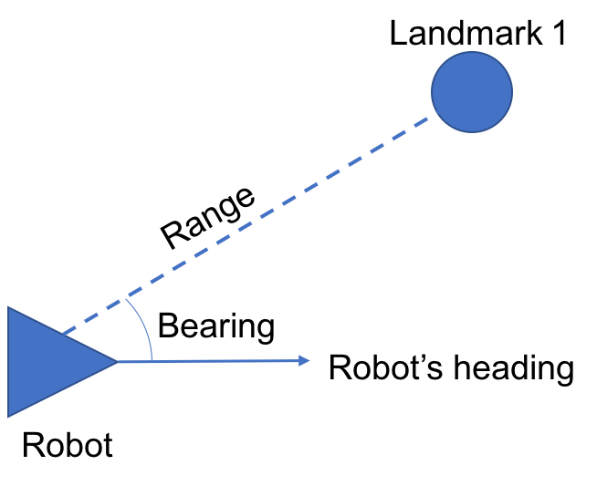

The Complete Algorithm

The code for the complete algorithm is shown below. It is very similar to the code for EKF localization with known correlation with state vector and covariance matrices that now include landmarks and with the update and measurement steps augmented as discussed above. Note also that after the states are estimated, in lines 157 through 167, the system calculates the sum of squared errors for both the robot positions and the landmark positions. This gives us a rough way to judge the quality of our filter tuning. I’ll go into a more principled method for Kalman filter tuning in a later post, but this works well enough for demonstration purposes.

addpath ../common;

deltaT = .02;
alphas = [.1 .01 .18 .08 0 0]; % motion model noise parameters

% measurement model noise parameters
Q_t = [11.8 0;
       0    .18];
   
n_robots = 1;
robot_num = 1;
n_landmarks = 15;
[Barcodes, Landmark_Groundtruth, Robots] = loadMRCLAMdataSet(n_robots);
[Robots, timesteps] = sampleMRCLAMdataSet(Robots, deltaT);

% add pose estimate matrix to Robots
Robots{robot_num}.Est = zeros(size(Robots{robot_num}.G,1), 4);

start = 600;
t = Robots{robot_num}.G(start, 1);

% initialize state mean with the groundtruth
% pose at timestep zero
stateMean = [Robots{robot_num}.G(start,2);
            Robots{robot_num}.G(start,3);
            Robots{robot_num}.G(start,4)];
        
% reshapes stateMean to 1x(2*n_landmarks+3)
% and remaps motion updates to new state vector
F_x = [eye(3) zeros(3, 2 * n_landmarks)];

stateMean = F_x' * stateMean;

% initialize diagonal of pose covariance with small, nonzero values
% since we have a good estimate of the starting pose
stateCov = zeros(2 * n_landmarks + 3, 2 * n_landmarks + 3);
stateCov(1:3,1:3) = 0.001;

% initialize landmark variances to large values since we have
% no prior information on the locations of the landmarks
for i = 4:n_landmarks * 2 + 3
    stateCov(i,i) = 10;
end
   
measurementIndex = 1;

% set up map between barcodes and landmark IDs
% barcode values are NOT the same as landmark IDs
codeDict = containers.Map(Barcodes(:,2),Barcodes(:,1));

% loop through all odometry and measurement samples
% updating the robot's pose estimate with each step
% reference table 10.1 in Probabilistic Robotics
for i = start:size(Robots{robot_num}.G, 1)
    
    % update time
    t = Robots{robot_num}.G(i, 1);
    
    % get control inputs at current timestep
    u_t = Robots{robot_num}.O(i, 2:end);
    % update robot bearing to last timestep's estimate
    theta = stateMean(3, 1);
    % calculate rotation and translation over last timestep
    rot = deltaT * u_t(2);
    halfRot = rot / 2;
    trans = u_t(1) * deltaT;
    
    % calculate pose update in world frame
    poseUpdate = [trans * cos(theta + halfRot);
                  trans * sin(theta + halfRot);
                  rot];
              
    % updated state mean and constrain bearing
    % to +/- pi
    stateMeanBar = stateMean + F_x' * poseUpdate;
    stateMeanBar(3) = conBear(stateMeanBar(3));
    
    % calculate movement jacobian
    g_t = [0 0 trans * -sin(theta + halfRot);
           0 0 trans * cos(theta + halfRot);
           0 0 0];
    G_t = eye(2 * n_landmarks + 3) + F_x' * g_t * F_x;
     
    % calculate motion covariance in control space
    M_t = [(alphas(1) * abs(u_t(1)) + alphas(2) * abs(u_t(2)))^2 0;
           0 (alphas(3) * abs(u_t(1)) + alphas(4) * abs(u_t(2)))^2];
       
    % calculate Jacobian to transform motion covariance to state space
    V_t = [cos(theta + halfRot) -0.5 * sin(theta + halfRot);
           sin(theta + halfRot) 0.5 * cos(theta + halfRot);
           0 1];
    
    % update state covariance
    R_t = V_t * M_t * V_t';
    stateCovBar = (G_t * stateCov * G_t') + (F_x' * R_t * F_x);
    
    % get measurements for current timestep
    [z, measurementIndex] = getObservations(Robots, robot_num, t, measurementIndex, codeDict);

    % if measurements are available
    if z(3,1) > 1
        S = zeros(size(z,2),3,3);
        zHat = zeros(2, size(z,2));
        % loop over every measurement and use to correct state estimate
        for k = 1:size(z, 2) 
            j = z(3,k);
            
            % if the landmark has never been seen before
            % add it to the state vector
            if stateMeanBar(j*2 + 2) == 0
                landmark_pos = [z(1,k) * cos(z(2,k) + stateMeanBar(3));
                                z(1,k) * sin(z(2,k) + stateMeanBar(3))];
                stateMeanBar(2*j+2:2*j+3) = [stateMeanBar(1) + landmark_pos(1);
                                             stateMeanBar(2) + landmark_pos(2)];
                continue;
            end

            % compute predicted range and bearing to the landmark
            delta = [stateMeanBar(2*j+2) - stateMeanBar(1);
                     stateMeanBar(2*j+3) - stateMeanBar(2)];
            q = delta' * delta;
            r = sqrt(q); % predicted range to landmark
            
            % predicted bearing to landmark
            pred_bear = conBear(atan2(delta(2), delta(1)) - stateMeanBar(3));
            % create predicted measurement
            zHat(:,k) = [r;
                         pred_bear];
            % calculate measurement Jacobian    
            h_t = [-delta(1)/r -delta(2)/r  0   delta(1)/r delta(2)/r;
                   delta(2)/q    -delta(1)/q    -1  -delta(2)/q  delta(1)/q];
                     
            F_1 = [eye(3); zeros(2,3)];
            F_2 = [zeros(3,2); eye(2)];
            F_xj = [F_1 zeros(5,2*j-2) F_2 zeros(5,2*n_landmarks - 2*j)];
            
            H_t = h_t * F_xj;
            
            % compute Kalman gain
            K = stateCovBar * H_t' / (H_t * stateCovBar * H_t' + Q_t);
            
            % incorporate new measurement into state mean and covariance
            stateMeanBar = stateMeanBar + K * (z(1:2,k) - zHat(:,k));
            stateCovBar = (eye(2*n_landmarks+3) - (K * H_t)) * stateCovBar;
        end
    end
    
    % update state mean and covariance
    stateMean = stateMeanBar;
    stateMean(3) = conBear(stateMean(3));
    stateCov = stateCovBar;
    
    % add new pose mean to estimated poses
    Robots{robot_num}.Est(i,:) = [t stateMean(1) stateMean(2) stateMean(3)];
end

% calculate land_loss: sum of squares of error in final landmark position
land_loss = 0;
for i = 1:n_landmarks
    x_diff = stateMean(2 * i + 1) - Landmark_Groundtruth(i, 2);
    y_diff = stateMean(2 * i + 2) - Landmark_Groundtruth(i, 3);
    sq_err = x_diff^2 + y_diff^2;
    land_loss = land_loss + sq_err;
end
disp(land_loss);

p_loss = path_loss(Robots, robot_num, start);
disp(p_loss);
animateMRCLAMdataSet(Robots, Landmark_Groundtruth, timesteps, deltaT);

Intro to the EKF Step 2: Localization With Unknown Correspondence

This tutorial is part of a series on Simultaneous Localization and Mapping (SLAM) using the extended Kalman filter. See the following for other tutorials in the series:

This tutorial will build incrementally on the previous tutorial: Localization With Known Correlation. We’re still just doing localization, which means the robot starts with a map of landmarks that does not change over the course of its run. The difference is this time when the robot gets a range and bearing measurement, it will not know to which landmark that measurement corresponds.

In this tutorial I will explain the process for estimating the correspondence between measurements and landmarks and present the correspondence algorithm on its own. Then I will show how the correspondence estimation algorithm can be integrated with the EKF localization algorithm introduced in the prior tutorial. As before, we’ll be using the UTIAS dataset for demonstration purposes.


Measurement Correspondence Intro

When our robot gets a measurement to a nearby landmark it can use that information to refine its estimate of its pose. In the last tutorial, each measurement received by our robot was in the form of z_t^i = [r_t^i\ \phi_t^i\ s_t^i]^T where z_t^i is the measurement to landmark i at time t. This vector contains the range r_t^i, bearing \phi_t^i, and, crucially, identity of the landmark being measured s_t^i. This could be interpreted as “landmark s is r meters away, at a bearing of \phi radians.”

In our current problem, the measurement vector will be z_t^i=[r_t^i\ \phi_t^i]^T. So we are no longer directly telling the robot to which landmark each measurement corresponds. Without knowledge of this correspondence measurements are basically useless to our robot. Sure, it knows the location of a landmark relative to its own location. But without knowing where that landmark is in the world it can’t use that information to refine its estimate of its pose.

So our robot needs a way to estimate the correspondence between its measurements and the landmarks in its map. One way it can do this is through maximum likelihood data association.


Maximum Likelihood Data Association

In maximum likelihood data association, as presented in section 7.5.2 of Probabilistic Robotics, the robot computes the probability that its current measurement corresponds to every landmark in its map. It then chooses the landmark with the highest probability of correspondence and assumes it is the correct association. This can be written as

\hat{c}_t = \text{argmax}_c\ p(z_t|c_{1:t},\ m,\ z_{1:t-1},\ u_{1:t})

In other words, given the robot’s past measurement correspondences c_{1:t}, map m, past measurements z_{1:t-1}, and past control inputs u_{1:t}, which landmark has the highest probability of producing measurement z_t?

In practice we find this by calculating the expected measurement and measurement covariance for every landmark in the map. We can then use these to calculate the measurement probability for every landmark and then select the landmark with the highest probability. The algorithm goes as follows:

    \begin{align*} \text{for all}&\text{ measurements } z_t^i=[r_t^i\ \phi_t^i]^T \text{ do} \\ \text{for}&\text{ all landmarks } k \text{ in the map } m \text{ do} \\ &q = (m_{k,x} - \bar{\mu}_{t,x})^2 + (m_{k,y} - \bar{\mu}_{t,y})^2 \\ &\hat{z}_t^k = \begin{bmatrix} \sqrt{q} \\ \text{atan2}(m_{k,y}-\bar{\mu}_{t,y},\ m_{k,x}-\bar{\mu}_{t,x})-\bar{\mu}_{t,\theta} \end{bmatrix} \\ &H_t^k = \begin{bmatrix} -\frac{m_{k,x}-\bar{\mu}_{t,x}}{\sqrt{q}} & -\frac{m_{k,y}-\bar{\mu}_{t,y}}{\sqrt{q}} & 0 \\ \frac{m_{k,y}-\bar{\mu}_{t,y}}{q} & -\frac{m_{k,x}-\bar{\mu}_{t,x}}{q} & -1\end{bmatrix} \\ &S_t^k = H_t^k \bar{\Sigma}_t [H_t^k]^T + Q_t \\ \text{end}&\text{for} \\ j(i) &= \text{argmax}_k\ \text{det}(2\pi S_t^k)^{-\frac{1}{2}} \text{exp}\{-\frac{1}{2}(z_t^i-\hat{z}_t^k)[S_t^k]^{-1}(z_t^i-\hat{z}_t^k)^T\}\\ \text{endfor}& \end{align*}

The end result j(i) is the estimated correspondence j for each measurement i. It should be noted that the probability estimates are conditioned on past correspondences. However, this method assumes that the past estimates are correct. This means that the correspondence estimates are very sensitive to incorrect associations; incorrect estimates are likely to remain incorrect on subsequent measurements. This makes the maximum likelihood method brittle and likely to diverge when measurements are incorrectly associated.

There are alternative methods that are more robust to incorrect associations. Multi-Hypothesis Tracking is one of these, but the maximum likelihood method is the simplest. For an introduction I think the maximum likelihood method is sufficient.


The Complete Algorithm

The code for the complete algorithm is shown below. It is the same as the code for EKF localization with known correlation with the addition of the maximum likelihood algorithm for measurement correspondence (lines 85 to 120). Note also that the code rendering program I’m using doesn’t seem to handle MATLAB code very well, and some of the highlighting is a little messed up.

addpath ../common;

deltaT = .02;
alphas = [.2 .03 .09 .08 0 0]; % motion model noise parameters

% measurement model noise parameters
sigma_range = .43;
sigma_bearing = .6;

Q_t = [sigma_range^2 0;
       0 sigma_bearing^2];

n_robots = 1;
robot_num = 1;
n_landmarks = 15;
[Barcodes, Landmark_Groundtruth, Robots] = loadMRCLAMdataSet(n_robots);
[Robots, timesteps] = sampleMRCLAMdataSet(Robots, deltaT);

% add pose estimate matrix to Robots
Robots{robot_num}.Est = zeros(size(Robots{robot_num}.G,1), 4);

start = 1; 
t = Robots{robot_num}.G(start, 1); 
% need mean and covariance for the initial pose estimate
poseMean = [Robots{robot_num}.G(start,2);
            Robots{robot_num}.G(start,3);
            Robots{robot_num}.G(start,4)];
poseCov = 0.01*eye(3);
       
measurementIndex = 1;

% set up map between barcodes and landmark IDs
codeDict = containers.Map(Barcodes(:,2),Barcodes(:,1));

while (Robots{robot_num}.M(measurementIndex, 1) < t - .05)
        measurementIndex = measurementIndex + 1;
end

% loop through all odometry and measurement samples
% updating the robot's pose estimate with each step
% reference table 7.3 in Probabilistic Robotics
for i = start:size(Robots{robot_num}.G, 1)
    theta = poseMean(3, 1);
    % update time
    t = Robots{robot_num}.G(i, 1);
    % update movement vector
    u_t = [Robots{robot_num}.O(i, 2); Robots{robot_num}.O(i, 3)];

    rot = deltaT * u_t(2);
    halfRot = rot / 2;
    trans = u_t(1) * deltaT;
    
    % calculate the movement Jacobian
    G_t = [1 0 trans * -sin(theta + halfRot);
           0 1 trans * cos(theta + halfRot);
           0 0 1];
    % calculate motion covariance in control space
    M_t = [(alphas(1) * abs(u_t(1)) + alphas(2) * abs(u_t(2)))^2 0;
           0 (alphas(3) * abs(u_t(1)) + alphas(4) * abs(u_t(2)))^2];
    % calculate Jacobian to transform motion covariance to state space
    V_t = [cos(theta + halfRot) -0.5 * sin(theta + halfRot);
           sin(theta + halfRot) 0.5 * cos(theta + halfRot);
           0 1];
    
    % calculate pose update from odometry
    poseUpdate = [trans * cos(theta + halfRot);
                  trans * sin(theta + halfRot);
                  rot];
    
    poseMeanBar = poseMean + poseUpdate;
    poseCovBar = G_t * poseCov * G_t' + V_t * M_t * V_t';
    
    % get measurements
    [z, measurementIndex] = getObservations(Robots, robot_num, t, measurementIndex, codeDict);
    
    % remove landmark ID from measurement because
    % we're trying to live without that
    z = z(1:2,:);
    
    % if features are observed
    % loop over all features and compute Kalman gain
    if z(1,1) > 0.1
        for k = 1:size(z, 2) % loop over every observed landmark
            
            % loop over all landmarks and compute MLE correspondence
            predZ = zeros(n_landmarks, 1, 2); % predicted measurements
            predS = zeros(n_landmarks, 2, 2); % predicted measurement covariances
            predH = zeros(n_landmarks, 2, 3); % predicted measurement Jacobians
            maxJ = 0; 
            landmarkIndex = 0;
            for j = 1:n_landmarks
                xDist = Landmark_Groundtruth(j, 2) - poseMeanBar(1);
                yDist = Landmark_Groundtruth(j, 3) - poseMeanBar(2);
                q = xDist^2 + yDist^2;
                
                % calculate predicted measurement
                predZ(j,:,:) = [sqrt(q);
                            conBear(atan2(yDist, xDist) - poseMeanBar(3))];
                        
                % calculate predicted measurement Jacobian
                predH(j,:,:) = [-xDist/sqrt(q) -yDist/sqrt(q) 0;
                                yDist/q        -xDist/q      -1];
                            
                % calculate predicted measurement covariance
                predS(j,:,:) = squeeze(predH(j,:,:)) * poseCovBar ...
                               * squeeze(predH(j,:,:))' + Q_t;
                
                % calculate probability of measurement correspondence          
                thisJ = det(2 * pi * squeeze(predS(j,:,:)))^(-0.5) * ...
                        exp(-0.5 * (z(:,k) - squeeze(predZ(j,:,:)))' ...
                        * inv(squeeze(predS(j,:,:))) ...
                        * (z(:,k) - squeeze(predZ(j,:,:))));
                
                % update correspondence if the probability is
                % higher than the previous maximum
                if thisJ > maxJ
                    maxJ = thisJ;
                    landmarkIndex = j;
                end
            end

            % compute Kalman gain
            K = poseCovBar * squeeze(predH(landmarkIndex,:,:))' ...
                * inv(squeeze(predS(landmarkIndex,:,:)));

            % update pose mean and covariance estimates
            poseMeanBar = poseMeanBar + K * (z(:,k) - squeeze(predZ(landmarkIndex,:,:)));
            poseCovBar = (eye(3) - (K * squeeze(predH(landmarkIndex,:,:)))) * poseCovBar;
        end
    end
    
    % update pose mean and covariance
    poseMean = poseMeanBar;
    poseMean(3) = conBear(poseMean(3));
    poseCov = poseCovBar;
    
    % add pose mean to estimated position vector
    Robots{robot_num}.Est(i,:) = [t poseMean(1) poseMean(2) poseMean(3)];
    
    % calculate error between mean pose and groundtruth 
    % for testing only
    %{
    groundtruth = [Robots{robot_num}.G(i, 2); 
                   Robots{robot_num}.G(i, 3); 
                   Robots{robot_num}.G(i, 4)];
    error = groundtruth - poseMean;
    %}
   
end
animateMRCLAMdataSet(Robots, Landmark_Groundtruth, timesteps, deltaT);

Intro to the EKF Step 1: Localization With Known Correlation

This tutorial is part of a series on Simultaneous Localization and Mapping (SLAM) using the extended Kalman filter. See the following for other tutorials in the series:

In this tutorial I’ll focus on one of the easiest state estimation problems: localization with known measurement correspondence. The “localization” part means that the robot already knows the positions of all of the landmarks in the environment. The “known correspondence” part means that when the robot measures the range and bearing to a landmark it always knows which landmark it’s measuring.

In this tutorial I’ll explain the EKF algorithm and then demonstrate how it can be implemented using the UTIAS dataset. I’ll break it down into the following sections:


Intro To The Algorithm

First off, why do we need this complicated algorithm for localization? Can’t we just track our position with odometry? This isn’t possible because a robot’s pose over time is not deterministic; it can’t be calculated exactly due to errors (also referred to as noise) in the odometry which accumulate over time.

This is why the Kalman filter represents the robot’s pose at time t as a multivariate normal probability distribution with a mean at \mu_t and covariance of \Sigma_t. The robot’s expected (or most likely) pose is at \mu_t and the uncertainty of that pose is quantified by \Sigma_t. The Kalman filter updates the robot’s pose using the robot’s motion from odometry u_t. Then it corrects for noise in the motion update using the robot’s sensor readings z_t.

One important advantage of the Kalman filter (and other similar algorithms) is that it is recursive. It only requires information about the state of the robot at time t-1 in order to estimate the state at time t. In other words, it doesn’t require information about any of the prior states of the robot from time t_0 to time t-2. This means it requires less memory and processor time to compute!

Below I present a mathematical definition for the extended Kalman filter. Most of it is taken from table 7.2 of Probabilistic Robotics by Thrun, Fox, and Burgard. It will be helpful to follow along in Probabilistic Robotics in addition to this tutorial. I’d also recommend reading chapter 3 of that book to gain a better understanding of Gaussian filters and recursive estimation.

Top of page


Inputs

  • the mean of the pose estimate from the previous timestep: \mu_{t-1} = \begin{bmatrix} x_{t-1} &y_{t-1} &\theta_{t-1} \end{bmatrix}^T
    • x_{t-1} is the robot’s previous x position in meters
    • y_{t-1} is the robot’s previous y position in meters
    • \theta_{t-1} is the robot’s previous heading in radians
  • the covariance matrix of the previous timestep, \Sigma_{t-1}
    • this represents the uncertainty of the pose estimate
  • the control inputs (or odometry) at the current timestep, u_t=\begin{bmatrix} v_t &\omega_t \end{bmatrix}^T
    • v_t is the robot’s linear velocity in meters/sec
    • \omega_t is the robot’s angular velocity in radians/sec
  • the measurements from the current timestep, z_t = \begin{bmatrix} z_t^1 &z_t^2 &\dots &z_t^k \end{bmatrix} where k is the number of measurements at time t
    • each z_t^i = \begin{bmatrix} r_t^i &\phi_t^i &s_t^i \end{bmatrix}^T where
      • r_t^i is the range to landmark i in meters
      • \phi_t^i is the bearing to landmark i in radians
      • s_t^i is the ID of landmark i
  • c_t is the correspondence between the measurement and landmarks
    • for our purposes this will be ignored for now
  • the map m = \begin{bmatrix}m_1 &m_2 &\dots &m_n \end{bmatrix} where n is the number of landmarks
    • each m_i = \begin{bmatrix} m_{i,x} &m_{i,y} &m_{i,s} \end{bmatrix}^T where
      • m_{i,x} is the x position of landmark i in meters
      • m_{i,y} is the y position of landmark i in meters
      • m_{i,s} is the ID of landmark i

Top of page


Outputs

  • the updated pose estimate, \mu_t
  • the updated covariance matrix, \Sigma_t
  • the measurement probability, p_{z_t}, which is the likelihood of the measurements z_t given the robot’s estimated pose before measurements were incorporated: \bar{\mu}_t
    • We’ll be ignoring this for now as well

Top of page


Algorithm

    \begin{flalign*} \text{Loc} &\text{alization with known correspondence}(\mu_{t-1}, \Sigma_{t-1},u_t,z_t,c_t,m): \\ &\theta = u_{t-1,\theta} \\ &G_t = \begin{bmatrix} 1 &0 &-v_t \Delta t \sin(\theta + \frac{\omega_t \Delta t}{2})\\ 0 &1 &v_t \Delta t \cos(\theta + \frac{\omega_t \Delta t}{2})\\ 0 &0 &1 \end{bmatrix} \\ &V_t = \begin{bmatrix} \cos(\theta + \frac{\omega_t \Delta t}{2}) &-\frac{1}{2} \sin(\theta + \frac{\omega_t \Delta t}{2}) \\ \sin(\theta + \frac{\omega_t \Delta t}{2}) &\frac{1}{2} \cos(\theta + \frac{\omega_t \Delta t}{2}) \\ 0 &1 \end{bmatrix} \\ &M_t = \begin{bmatrix} \alpha_1 v_{t}^{2} + \alpha_2 \omega_{t}^{2} &0 \\ 0 &\alpha_{3} v_{t}^{2} + \alpha_4 \omega_{t}^{2} \end{bmatrix} \\ &\bar{\mu_t} = \mu_{t-1} + \begin{bmatrix} v_t \Delta t \cos(\theta + \frac{\omega_t \Delta t}{2}) \\ v_t \Delta t \sin(\theta + \frac{\omega_t \Delta t}{2}) \\ \omega_t \Delta t \end{bmatrix} \\ &\bar{\Sigma}_t = G_t \Sigma_{t-1} G_{t}^{T} + V_t M_t V_{t}^{T} \\ &Q_t = \begin{bmatrix} \sigma_{r}^{2} &0 &0 \\ 0 &\sigma_{\phi}^{2} &0 \\ 0 &0 &\sigma_{s}^{2} \end{bmatrix}\\ &\text{for all observed features $z_{t}^{i}=\begin{bmatrix} r_{t}^{i} &\phi_{t}^{i} &s_{t}^{i}\end{bmatrix}^T$ do} \\ \end{flalign*}

    \begin{flalign*} &j=c_{t}^{i}\\ &q = (m_{j,x} - \bar{\mu}_{t,x})^2 + (m_{j,y} - \bar{\mu}_{t,y})^2 \\ &\hat{z}_{t}^{i} = \begin{bmatrix} \sqrt{q} \\ \text{atan2}(m_{j,y} - \bar{\mu}_{t,y} \text{,  }m_{j,x} - \bar{\mu}_{t,x}) - \bar{\mu}_{t, \theta} \\ m_{j,s} \end{bmatrix} \\ &H_{t}^{i} = \begin{bmatrix} -\frac{m_{j,x} - \bar{\mu}_{t,x}}{\sqrt{q}} & -\frac{m_{j,y} - \bar{\mu}_{t,y}}{\sqrt{q}} &0 \\ \frac{m_{j,y} - \bar{\mu}_{t,y}}{q} &-\frac{m_{j,x} - \bar{\mu}_{t,x}}{q} &-1 \\ 0 &0 &0 \end{bmatrix} \\ &S_{t}^{i} = H_{t}^{i} \bar{\Sigma}_t \lbrack H_{t}^{i} \rbrack ^T + Q_t \\ &K_{t}^{i} = \bar{\Sigma}_t \lbrack H_{t}^{i} \rbrack ^T \lbrack S_{t}^{i} \rbrack ^{-1} \\ &\bar{\mu}_t = \bar{\mu}_t + K_{t}^{i}(z_{t}^{i} - \hat{z}_{t}^{i}) \\ &\bar{\Sigma}_t = (I - K_{t}^{i} H_t^i) \bar{\Sigma}_t \\ \end{flalign*}

    \begin{flalign*} &\text{end for} \\ &\mu_t = \bar{\mu}_t \\ &\Sigma_t = \bar{\Sigma}_t \\ &p_{z_t} = \prod_i \det(2 \pi S_t^i)^{-\frac{1}{2}} \exp \{ -\frac{1}{2}(z_t^i - \hat{z}_t^i)^T \lbrack S_t^i \rbrack ^{-1} (z_t^i - \hat{z}_t^i) \} \\ &\text{return } \mu_t, \Sigma_t, p_{z_t} \\ \end{flalign*}

Top of page


Motion Update

The algorithm is divided into two parts: the motion update and the sensor update. First, in the motion update the odometry information is incorporated into the state estimate. The motion update is based around a motion model g(u_t, x_{t-1}), which calculates a new pose based on the previous pose x_{t-1} and the odometry u_t.

(1)   \begin{equation*} \bar{\mu_t} = g(u_t, x_{t-1}) = \mu_{t-1} + \begin{bmatrix} v_t \Delta t \cos(\theta + \frac{\omega_t \Delta t}{2}) \\ v_t \Delta t \sin(\theta + \frac{\omega_t \Delta t}{2}) \\ \omega_t \Delta t \end{bmatrix} \end{equation*}

In this equation \bar{\mu}_t denotes the estimated updated mean of the pose distribution. The motion model I’m using assumes that the robot rotates in place, then drives in a straight line, then rotates in place again. This is a common approximation and it’s accurate enough as long as \Delta t is small.

In addition to calculating a new mean for our robot’s pose distribution \bar{\mu}_t we need calculate an estimated covariance for the new pose, \bar{\Sigma}_t. In order to do this we need to multiply the covariance from the last timestep, \Sigma_{t-1}  by the derivative (also called the Jacobian) of the motion model with respect to the previous state x_{t-1}:

(2)   \begin{equation*} G_t = \frac{\partial g(u_t, \mu_{t-1})}{\partial x_{t-1}} = \begin{bmatrix} 1 &0 &-v_t \Delta t \sin(\theta + \frac{\omega_t \Delta t}{2})\\ 0 &1 &v_t \Delta t \cos(\theta + \frac{\omega_t \Delta t}{2})\\ 0 &0 &1 \end{bmatrix} \end{equation*}

The multiplication looks like the following: G_t \Sigma_{t-1} G_t^T. We also need to calculate the additional noise (or uncertainty) associated with the motion that occurred between t-1 and t.

(3)   \begin{equation*} M_t = \begin{bmatrix} \alpha_1 v_{t}^{2} + \alpha_2 \omega_{t}^{2} &0 \\ 0 &\alpha_{3} v_{t}^{2} + \alpha_4 \omega_{t}^{2} \end{bmatrix} \end{equation*}

The alphas \alpha_1 through \alpha_4 are noise parameters that, unfortunately, need to be hand-tuned for the particular robot being used. Also, M_t is in control space and we need to map it into state space. To do this we need the Jacobian of the motion model with respect to the motion parameters u_t:

(4)   \begin{equation*} V_t = \frac{\partial g(u_t, \mu_{t-1})}{\partial u_t} = \begin{bmatrix} \cos(\theta + \frac{\omega_t \Delta t}{2}) &-\frac{1}{2} \sin(\theta + \frac{\omega_t \Delta t}{2}) \\ \sin(\theta + \frac{\omega_t \Delta t}{2}) &\frac{1}{2} \cos(\theta + \frac{\omega_t \Delta t}{2}) \\ 0 &1 \end{bmatrix} \end{equation*}

So we can map the noise M_t to state space with the following multiplication: V_t M_t V_t^T. To get the complete updated covariance \bar{\Sigma}_t we add the transformed covariance from the previous timestep to the additional noise:

(5)   \begin{equation*} \bar{\Sigma}_t = G_t \Sigma_{t-1} G_{t}^{T} + V_t M_t V_{t}^{T} \end{equation*}

So the motion update step updates the robot’s pose mean and covariance based on its odometry. You may have noticed, however, that the covariance only gets larger in this step. This means our uncertainty about the robot’s pose always grows when we incorporate odometry. We can decrease the uncertainty by incorporating sensor information, which is what we do in the next step.

Note: The motion model and associated Jacobians presented in the preceding section are different from those presented in Probabilistic Robotics. The model presented in Probabilistic Robotics assumes that the robot is always moving in an arc and its angular velocity, \omega_t, is never zero. The Jacobians for this model involve dividing by \omega_t. This means that the model breaks if \omega_t is ever equal to zero. This is a problem for us because \omega_t often is equal to zero in the UTIAS dataset. That is why I subbed in my own motion model.

Top of page


Sensor Update

The sensor update refines the robot’s pose estimate and decreases its uncertainty. This happens in the for loop of the algorithm. It is run for every measurement that occurs at timestep t.

In the first step of the sensor update we calculate what the range and bearing to the landmark would have been if the estimated pose mean \bar{\mu}_t were correct. This is called the expected measurement \hat{z}_t and it is calculated using the measurement model h_t(x_t,m).

(6)   \begin{equation*} q = (m_{j,x} - \bar{\mu}_{t,x})^2 + (m_{j,y} - \bar{\mu}_{t,y})^2 \end{equation*}

(7)   \begin{equation*} \hat{z}_{t}^{i} = h(x_t, m) = \begin{bmatrix} \sqrt{q} \\ \text{atan2}(m_{j,y} - \bar{\mu}_{t,y} \text{,  }m_{j,x} - \bar{\mu}_{t,x}) - \bar{\mu}_{t, \theta} \\ m_{j,s} \end{bmatrix} \\ \end{equation*}

Remember that m_{j,x}, m_{j,y}, and m_{j,s} are the x position, y position, and ID of landmark j, respectively.

We also need to calculate the additional noise associated with the measurement. To do this we need the Jacobian of the measurement model with respect to the robot’s pose:

(8)   \begin{equation*} H_{t}^{i} = \frac{\partial h(\bar{\mu}_t, m)}{\partial x_t} = \begin{bmatrix} -\frac{m_{j,x} - \bar{\mu}_{t,x}}{\sqrt{q}} & -\frac{m_{j,y} - \bar{\mu}_{t,y}}{\sqrt{q}} &0 \\ \frac{m_{j,y} - \bar{\mu}_{t,y}}{q} &-\frac{m_{j,x} - \bar{\mu}_{t,x}}{q} &-1 \\ 0 &0 &0 \end{bmatrix} \end{equation*}

The measurement noise is calculated by multiplying the prior estimated covariance with the measurement model Jacobian and adding additional noise for the new measurement. The additional noise Q_t is a constant for all measurements. It is a 3 \times 3 diagonal matrix with noise parameters \sigma_r, \sigma_\phi, and \sigma_s. The sigmas represent the noise for landmark range, bearing, and noise, respectively. Like the alphas in equation (3), the sigmas must be hand-tuned in order to obtain good performance.

(9)   \begin{equation*} S_t^i = H_t^i \bar{\Sigma}_t \lbrack H_t^i \rbrack ^T + Q_t \end{equation*}

S_t^i is then used to calculate the Kalman gain, K_t^i. The Kalman gain determines how heavily the sensor information should be weighted when correcting the estimated new pose \bar{\mu}_t and \bar{\Sigma}_t.

(10)   \begin{equation*} K_{t}^{i} = \bar{\Sigma}_t \lbrack H_{t}^{i} \rbrack ^T \lbrack S_{t}^{i} \rbrack ^{-1} \end{equation*}

The Kalman gain is used to update the estimated pose mean and covariance \bar{\mu}_t and \bar{\Sigma}_t as follows:

(11)   \begin{equation*} \bar{\mu}_t = \bar{\mu}_t + K_{t}^{i}(z_{t}^{i} - \hat{z}_{t}^{i}) \end{equation*}

(12)   \begin{equation*} \bar{\Sigma}_t = (I - K_{t}^{i} H_t^i) \bar{\Sigma}_t \end{equation*}

The amount of correction to the estimated pose mean depends on K_t^i and the difference between the expected measurement \hat{z}_t^i (calculated in equation (7) and the actual measurement z_t^i. A larger discrepancy between the expected and actual measurement will result in a larger correction.

After the sensor update is complete the pose mean and covariance are updated with the estimated values: \mu_t = \bar{\mu}_t and \Sigma_t = \bar{\Sigma}_t. The measurement probability is also calculated here but we are not making use of this value.

Top of page


Code

When writing robotics software I’m often frustrated by the separation between theory and software engineering. There are many good theoretical explanations of the extended Kalman filter online. There are also several good examples of code that uses an EKF. But I was unable to find any textbook, academic paper, blog post, or stackexchange thread that did a good job of demonstrating how the math translates into code. I’m hoping my code below will change that. I’ve been careful to explain all major steps and refer to the equations above in the comments. I hope you find it helpful!

Lastly, note that comments in MATLAB begin with a % symbol. The code rendering plugin I used doesn’t seem to get this when highlighting the code, however. So be aware that the highlighting below isn’t always accurate, but the actual code is.

addpath ../common; % adds support functions used in all my EKF programs
                   % check my github for details

deltaT = .02; 
alphas = [.2 .03 .09 .08 0 0]; % robot-dependent motion noise parameters
                               % see equation 3

% robot-dependent sensor noise parameters
% see equation 9
sigma_range = 2;
sigma_bearing = 3;
sigma_id = 1;

Q_t = [sigma_range^2 0 0;
       0 sigma_bearing^2 0;
       0 0 sigma_id^2];

measurement_prob = 0;
n_robots = 1;
robot_num = 1;

% load and resample raw data from UTIAS data set
% The robot's position groundtruth, odometry, and measurements 
% are stored in Robots
[Barcodes, Landmark_Groundtruth, Robots] = loadMRCLAMdataSet(n_robots);
[Robots, timesteps] = sampleMRCLAMdataSet(Robots, deltaT);

% add pose estimate matrix to Robots
% data will be added to this as the program runs
Robots{robot_num}.Est = zeros(size(Robots{robot_num}.G,1), 4);

% initialize time, and pose estimate
start = 600; % start index is set to 600 because earlier data was 
             % found to cause problems
t = Robots{robot_num}.G(start, 1); % set start time

% set starting pose mean to pose groundtruth at start time
poseMean = [Robots{robot_num}.G(start,2);
            Robots{robot_num}.G(start,3);
            Robots{robot_num}.G(start,4)];
poseCov = [0.01 0.01 0.01;
           0.01 0.01 0.01;
           0.01 0.01 0.01];
       
% tracks which measurement is next received
measurementIndex = 1;

% set up map between barcodes and landmark IDs
codeDict = containers.Map(Barcodes(:,2),Barcodes(:,1));

% advance measurement index until the next measurement time 
% is greater than the starting time
while (Robots{robot_num}.M(measurementIndex, 1) < t - .05)
        measurementIndex = measurementIndex + 1;
end

% loop through all odometry and measurement samples
% updating the robot's pose estimate with each step
% reference table 7.2 in Probabilistic Robotics
for i = start:size(Robots{robot_num}.G, 1)
    theta = poseMean(3, 1);
    % update time
    t = Robots{robot_num}.G(i, 1);
    % update movement vector per equation 1
    u_t = [Robots{robot_num}.O(i, 2); Robots{robot_num}.O(i, 3)];

    rot = deltaT * u_t(2);
    halfRot = rot / 2;
    trans = u_t(1) * deltaT;
    
    % calculate the movement Jacobian per equation 2
    G_t = [1 0 trans * -sin(theta + halfRot);
           0 1 trans * cos(theta + halfRot);
           0 0 1];
    % calculate motion covariance in control space per equation 3
    M_t = [(alphas(1) * abs(u_t(1)) + alphas(2) * abs(u_t(2)))^2 0;
           0 (alphas(3) * abs(u_t(1)) + alphas(4) * abs(u_t(2)))^2];
       
    % calculate Jacobian to transform motion covariance to state space
    % per equation 4
    V_t = [cos(theta + halfRot) -0.5 * sin(theta + halfRot);
           sin(theta + halfRot) 0.5 * cos(theta + halfRot);
           0 1];
    
    % calculate pose update
    poseUpdate = [trans * cos(theta + halfRot);
                  trans * sin(theta + halfRot);
                  rot];
              
    % calculate estimated pose mean per equation 1
    poseMeanBar = poseMean + poseUpdate;
    % calculate estimated pose covariance per equation 5
    poseCovBar = G_t * poseCov * G_t' + V_t * M_t * V_t';
    
    
    % get measurements for the current timestep, if any exist
    [z, measurementIndex] = getObservations(Robots, robot_num, t, measurementIndex, codeDict);
    
    % create two matrices for expected measurement and measurement
    % covariance
    S = zeros(size(z,2),3,3);
    zHat = zeros(3, size(z,2));
    
    % if any measurements are available
    if z(3,1) > 1
        for k = 1:size(z, 2) % loop over every measurement
            j = z(3,k);

            % get coordinates of the measured landmark
            m = Landmark_Groundtruth(j, 2:3);

            % compute the expected measurement per equations 6 and 7
            xDist = m(1) - poseMeanBar(1);
            yDist = m(2) - poseMeanBar(2);
            q = xDist^2 + yDist^2;
            
            % constrains expected bearing to between 0 and 2*pi
            pred_bear = conBear(atan2(yDist, xDist) - poseMeanBar(3));
            
            zHat(:,k) = [sqrt(q);
                         pred_bear;
                         j];

            % calculate Jacobian of the measurement model per equation 8
            H = [(-1 * (xDist / sqrt(q))) (-1 * (yDist / sqrt(q))) 0;
                 (yDist / q) (-1 * (xDist / q)) -1;
                 0 0 0];
             
            % compute S per equation 9
            S(k,:,:) = H * poseCovBar * H' + Q_t;

            % compute Kalman gain per equation 10
            K = poseCov * H' * inv(squeeze(S(k,:,:)));
                
            % update pose mean and covariance estimates
            % per equations 11 and 12
            poseMeanBar = poseMeanBar + K * (z(:,k) - zHat(:,k));
            poseCovBar = (eye(3) - (K * H)) * poseCovBar;
        end
    end
    
    % update pose mean and covariance
    % constrains heading to between 0 and 2*pi
    poseMean = poseMeanBar;
    poseMean(3) = conBear(poseMean(3));
    poseCov = poseCovBar;
    
    % add pose mean to estimated position vector
    Robots{robot_num}.Est(i,:) = [t poseMean(1) poseMean(2) poseMean(3)];
    
    % calculate error between mean pose and groundtruth
    % for testing only
    %{
    groundtruth = [Robots{robot_num}.G(i, 2); 
                   Robots{robot_num}.G(i, 3); 
                   Robots{robot_num}.G(i, 4)];
    error = groundtruth - poseMean;
    %}
   
end

% display results!
animateMRCLAMdataSet(Robots, Landmark_Groundtruth, timesteps, deltaT);

Note: My tuning of the noise parameters in the code below is workable. But I didn’t spend as much time on them as I did for subsequent iterations of this tutorial. If you’d like to play with them I’m sure you can improve on my tunings!

Top of page

Intro to the EKF Step 0: The Data

This post is part of a series on SLAM with the extended Kalman filter. For other posts in the series see below.

Intro To The UTIAS Dataset

Writing programs for actual robots is difficult. Robots are expensive, testing code takes a lot of time, and the results are often difficult to interpret. This is why we don’t do most of our software development on actual robots. Instead it is much easier to run the actual robot once and log all of the robot’s sensor data, command inputs, and other relevant data. This way we can test our software on the logged data in a few seconds rather than doing a new test run every time we make a change to our code.

Setup used to make the UTIAS dataset

However, it’s difficult to make our own datasets for localization and mapping. In order to evaluate the accuracy of our SLAM software we need to know the actual (or groundtruth) pose of the robot with high accuracy at all times. This requires the use of motion capture setups which are well beyond the reach of most hobbyists. The good news is that university research groups routinely make their data sets available to the public. One such data set that is useful for our purposes is the UTIAS Multi-Robot Localization and Mapping (MRCLAM) dataset from the Autonomous Space Robotics Lab at the University of Toronto. I’ll refer to it as the UTIAS dataset for short.

The UTIAS data includes everything we’ll need to test our localization and mapping software: logs of the robot’s sensor data, accurate groundtruth poses for the robots throughout the run, and groundtruth positions for each landmark. I’ll go through each of those in detail below. You should take this opportunity download and extract “Dataset 1” from the download section of the MRCLAM webpage. You should also read the “Data Collection Details” of that page.


The Robots

The UTIAS dataset actually includes data from five different robots, all of which were run at the same time. This is because the dataset was originally intended for use in cooperative localization and mapping. However, this adds an unnecessary complication for our purposes. We will only be using the data from robot 1 in this tutorial.

The Measurements

The robot’s measurements are split up into two files: one for landmark measurements (Robot1_Measurements.dat) and one for odometry data (Robot1_Odometry.dat).

Illustration of a landmark measurement.

Each line of the Measurements file represents a measurement of a single landmark. We define a “measurement” with three quantities: range, the distance between the robot and the landmark in meters; bearing, the angle in radians between the landmark and the robot’s heading; and landmark ID, the unique identifier of the landmark being measured. Each line of the measurements file records the time the measurement occurred, the barcode for the landmark that was measured, the range, and the bearing. Note that the landmark barcode in the measurements file is not equivalent to the landmark ID in the landmark groundtruth file. The barcodes.dat file defines the mapping between the landmark barcodes and ID numbers.

The odometry file is pretty simple by comparison. Each line specifies the time, the robot’s linear velocity (in m/s), and its angular velocity (in rad/s).

The Groundtruth

Robot1_Groundtruth.dat specifies the robot’s actual pose in the global reference frame at any given time throughout the run. This is the part of the dataset that required the use of a motion capture system. Most of us could not recreate this on our own, so it’s nice that the University of Toronto made their data publicly available. Each line of the groundtruth file specifies the time, the robot’s x position in meters, the robot’s y position in meters, and the robot’s heading in radians.


The Landmarks

Landmark_Groundtruth.dat specifies the actual position of all of the landmarks in the environment. Each line specifies the landmark ID number, the x position, the y position, the standard deviation of the x position, and the std dev of the y position.


The Utilities

There are also a few useful MATLAB scripts available on the MRCLAM webpage.

loadMRCLAMdataSet.m will load the information in the .dat files into MATLAB variables. sampleMRCLAMdataSet.m will resample the data at 50Hz. This means that all of the measurements, odometry, and groundtruth information will come in at a predictable time interval. That will make things much easier. Lastly, animateMRCLAMdataSet.m will animate the motion of the robots throughout the run.

The problem with these scripts is they assume we want to work with all 5 robots. There are adapted versions of the scripts in my GitHub repo that only work with robot 1. Additionally, I adapted animateMRCLAMdataSet.m to animate both the groundtruth pose of robot 1 and the pose estimated by the EKF localization program. This will allow us to see just how well our program’s pose estimate tracks the robot’s true pose.

Intro to the Extended Kalman Filter

I started a PhD in computer science at CU Boulder four months ago. This is mainly because three years ago I made a wager. Since then I’ve become completely fascinated with robotics and have decided to pursue robotics research as a career.

Colin with his new sonar

Colin, my robot

I’m currently working at the ARPG at CU Boulder. As part of that work I wrote an implementation of SLAM using the Extended Kalman Filter (EKF). The EKF is the oldest probabilistic SLAM method. It’s a great introduction to SLAM techniques. However, it’s not very good by modern standards; it’s computationally expensive and it requires hand tuning several parameters to achieve passably accurate operation. But it is a good step in learning SLAM techniques, and I will likely implement an EKF on Colin at some point.

Tutorial Structure

Over the next several posts I’ll take you through my implementation of EKF SLAM in several steps. At the first step the robot will have a lot of prior knowledge about its environment and sensor readings. We’ll progressively take away pieces of the robot’s prior knowledge, making the task harder and harder as we go. In our last step the robot will have no prior knowledge. Our solution to this last step will be a fully-fledged SLAM program.

See the following for links to other tutorials in this series:

Dataset

I will use the UTIAS robot localization dataset for my tutorials. I’ll go into more detail on how to use and interpret the UTIAS data in my next post. The important thing to understand is that the UTIAS data abstracts away large parts of the SLAM problem such as controls and computer vision. This means we can just focus on programming and tuning our Extended Kalman Filters when using the UTIAS data. However, it also means we can’t simply upload our EKF programs to Colin. We would also need to write supporting programs that could supply data to the EKF in a form it can use.

Reference Material

Most of the math I’ll present in the next several posts came from Probabilistic Robotics, by Thrun, Fox, and Burgard. It’s a great book for anyone who wants to learn the theory behind fundamental robotics problems. It’s also not difficult to find a free pdf copy of an earlier edition if you don’t want to pay $85 for the current edition. But be warned that there are some math errors in the free pdf edition, so you may need to re-derive some things if you use it.

Probabilistic Robotics has a great section on Extended Kalman Filters and I’d recommend reading it thoroughly. However, the motion model it presents can’t be used with the UTIAS dataset so I’ll be using a different one. I’ll highlight where I deviate from the method presented in Probabilistic Robotics so as not to confuse those of you who are using it as a reference.

Programming Note

Lastly, the code I’m presenting is written in MATLAB. For those who don’t have access to MATLAB I would suggest using Python and NumPy. NumPy has all of the required functions to complete these tutorials. The only thing to watch out for is that Python uses zero-based indexing while MATLAB uses one-based indexing. If you don’t keep this in mind it could cause you some serious headaches.

Camera Pose Estimation Using Convolutional Neural Networks

It’s been quite a while since I last posted here. Since my last post I started a PhD in computer science at the University of Colorado, Boulder. I’ve been working on a lot of fun robotics-related stuff lately, but I haven’t had the time to work on Colin. However, I recently finished a really interesting project and I thought I’d take some time to do a quick write-up on it. The project really encapsulates what I’ve loved about my first semester in grad school. When I started I knew basically nothing about neural networks or pose estimation. But in just a few short weeks I had learned enough to build, train, and test a neural network for camera pose estimation. I absolutely love that this is my job now.

My project involved implementing the method for camera pose estimation presented in this paper. The basic idea is this: given two photos of the same scene taken from different positions we need to determine how the camera moved between those two photos. We must calculate both the translation and rotation in three dimensions. A good solution to this problem has many applications, but the one I’m most interested in is visual odometry, the process of determining a robot’s change in position using information from its camera.

For this post I describe how this problem is traditionally addressed. I then present the new method and compare it to the traditional methods. Lastly I present the code for my implementation of the new method. For the implementation section I assume you have some familiarity with Python 3 and Keras. If not there’s plenty of good tutorials on both. I didn’t know either about a month and a half ago. I also didn’t know anything about neural networks when I started this project. If you’re in the same boat I’d suggest you go through these notes and this tutorial. I found them very helpful.

The Traditional Approach
Using CNNs
Comparing Approaches
The Code

Challenge: compute the relative camera pose change between two photos of the same scene


The Traditional Approach


The normal approach to computing the relative pose change between two images involves feature matching. To be brief, a feature detector such as FAST is used to find “keypoints” in both input images. The algorithm assigns unique descriptors to each feature. Examples of possible descriptors are SIFT and BRIEF. The algorithm then compares the set of descriptors from each image to find the set of descriptors common to both images (the intersection of the two sets). Finally, the homography between the two sets of descriptors for the images is computed. This allows us to calculate the change in camera pose between the two images.

This approach is computationally intensive. Each feature descriptor must be compared to every other descriptor to find matches. Additionally, in order to perform well it must be able to find a large set of matching feature points between the two images. There are some cases where this is not possible, however. Scenes with few features will result in an insufficient number of features being detected. On the other hand, objects with very repetitive structure will have many similar features and the matching algorithm will find spurious correspondences between them. Lastly, if the change in camera pose between the images is too great, there may not be sufficient overlap between the sets of features from each image.

Feature Matching

Case in which feature matching is not able to find enough matching features for accurate pose estimation.


Using Convolutional Neural Networks


Because of the limitations of traditional feature-matching for relative camera pose estimation there have been several attempts to employ convolutional neural networks for this purpose.

The method presented in the subject paper is to feed each image into a separate branch of a Siamese neural network. A Siamese neural network contains two or more branches, or subnetworks. The architecture and weights of all the branches are identical. Siamese networks are adept at finding similarities or relationships between images. The structure of the Siamese branches for the network presented in this paper is the same as the convolutional section of AlexNet. AlexNet is a popular neural network for image classification.

The outputs from the Siamese branches are concatenated and then fed into a single fully-connected layer with 7 outputs. These outputs correspond to the 3D translation vector and the orientation quaternion required to move the camera from its initial pose to its final pose.

One additional interesting feature of this approach is that it applies a unique pooling technique between the convolutional and fully-connected sections of the network. Convolutional networks can theoretically accept inputs of arbitrary size. However, the fully connected layers at the end of a convolutional network require fixed-size input. Normally images are cropped or downsampled before being fed into the convolutional section of the network to ensure the input to the fully connected layers is the correct size. However, this can also result in a loss of information in the original image. Spatial pyramid pooling (SPP) generates a fixed-size representation from an arbitrary input size. This means that, by including an SPP layer between the convolutional and fully connected layers, we can give our network the ability to accept arbitrary-sized inputs. It also means that the convolutional section of the network is able to use all of the information present in the input images. The authors of this paper found that it significantly increased the accuracy of their model.


Comparing The Approaches


The performance of the convolutional neural network was compared to the OpenCV implementations of two feature matching methods: SURF and ORB. Images from the DTU robot image dataset were used to test all three methods. The DTU dataset was created by taking photos of several scenes using a camera positioned by a robotic arm. This means that we know the groundtruth for the change in camera pose with high accuracy. So evaluation of the accuracy of each method is quite simple. Additionally, it means the labels used for training the CNN are highly accurate.

Feature matching methods were, in general, more accurate. However, there are certain cases in which the neural network performs better. For higher changes in position and orientation the CNN can slightly outperform feature based methods. Also, the CNN can perform significantly better in cases where it is difficult to find and match features. For example, when the images do not contain a sufficient number of features.

Histogram of errors for orientation (left) and translation (right). The above histograms compare 4 different CNN architectures to SURF and ORB.


The Code

I’ve posted the Python 3 code for the neural network below. Supporting code for loading data from the image files and visualizing the results can be found on my github repository. Also, the image files themselves can be downloaded from the DTU website.

# camera-pose.py
# Andrew Kramer

# regresses the relative camera pose between two images using the method 
# presented in https://arxiv.org/pdf/1702.01381.pdf

import numpy as np
import tensorflow
import gzip
import sys
import pickle
import keras
import math
import os

from keras.models import Sequential, Model, load_model
from keras.layers import Dense, Dropout, Activation, Flatten
from keras.layers import Conv2D, MaxPooling2D, Input, Lambda
from keras.utils import np_utils
from keras.datasets import mnist
from keras import backend as K
from dataloader import DataLoader
from pooling.spp.SpatialPyramidPooling import SpatialPyramidPooling

beta = 10
epochs = 10

# define loss function for training the network
def custom_objective(y_true, y_pred):
	error = K.square(y_pred - y_true)
	transMag = K.sqrt(error[0] + error[1] + error[2])
	orientMag = K.sqrt(error[3] + error[4] + error[5] + error[6])
	return K.mean(transMag + (beta * orientMag))

def dot_product(v1, v2):
	return sum((a*b) for a,b in zip(v1,v2))

def length(v):
	return math.sqrt(dot_product(v,v))

def compute_mean_error(y_true, y_pred):
	trans_error = 0
	orient_error = 0
	for i in range(0,y_true.shape[0]):
		trans_error += math.acos(dot_product(y_true[i,:3], y_pred[i,:3])/
					(length(y_true[i,:3]) * length(y_pred[i,:3])))
		orient_error += math.acos(dot_product(y_true[i,3:], y_pred[i,3:])/
					 (length(y_true[i,3:]) * length(y_pred[i,3:])))
	mean_trans = trans_error / y_true.shape[0]
	mean_orient = orient_error / y_true.shape[0]
	return mean_trans, mean_orient

# define the architecture for the Siamese branches
def create_conv_branch(input_shape):
	model = Sequential()
	model.add(Conv2D(96, kernel_size=(11,11),
					 strides=4, padding='valid',
					 activation='relu',
					 input_shape=input_shape))
	model.add(MaxPooling2D(pool_size=(2,2), strides=2))
	model.add(Conv2D(256, kernel_size=(5,5),
					 strides=1, padding='same',
					 activation='relu'))
	model.add(MaxPooling2D(pool_size=(3,3), strides=1))
	model.add(Conv2D(384, kernel_size=(3,3),
					 strides=1, padding='same',
					 activation='relu'))
	model.add(Conv2D(384, kernel_size=(3,3),
					 strides=1, padding='same',
					 activation='relu'))
	model.add(Conv2D(256, kernel_size=(3,3),
					 strides=1, padding='same',
					 activation='relu'))
	model.add(SpatialPyramidPooling([1,2,3,6,13]))
	return model

if __name__ == "__main__":

	img_rows, img_cols = 227, 227
	category_IDs = list(range(1,25)) # category IDs from which to pull test and training data
	file_name = 'huge_model_spp_10epoch.h5'
	model = None
	# load training and testing data:
	loader = DataLoader(category_IDs, img_rows, img_cols)
	train_data, test_data = loader.get_data()
	train_labels, test_labels = loader.get_labels()
	input_shape = loader.get_input_shape()

	# define structure of convolutional branches
	conv_branch = create_conv_branch(input_shape)
	branch_a = Input(shape=input_shape)
	branch_b = Input(shape=input_shape)

	processed_a = conv_branch(branch_a)
	processed_b = conv_branch(branch_b)

	# concatenate the outputs of the CNN branches
	regression = keras.layers.concatenate([processed_a, processed_b])

	output = Dense(7, kernel_initializer='normal', name='output')(regression)
	model = Model(inputs=[branch_a, branch_b], outputs=[output])

	model.compile(loss=custom_objective, 
				  optimizer=keras.optimizers.Adam(lr=.0001, decay=.00001),
				  metrics=['accuracy'])

	if os.path.isfile(file_name):
		print("model", file_name, "found")
		model.load_weights(file_name)
		print("model loaded from file")
	else:
		model.fit([train_data[:,0], train_data[:,1]], train_labels,
				  batch_size=128,
				  epochs = epochs,
				  validation_split=0.1,
				  shuffle=True)
		model.save_weights(file_name)
		print("model saved as file", file_name)

	pred = model.predict([test_data[:,0], test_data[:,1]])
	test_trans, test_orient = compute_mean_error(pred, test_labels)
	np.savetxt('pred_spp.txt', pred, delimiter=' ')
	np.savetxt('labels_spp.txt', test_labels, delimiter=' ')

	print('*     Mean translation error on test set: %0.2f' % (test_trans))
	print('*     Mean orientation error on test set: %0.2f' % (test_orient))