Beyond EKF SLAM

My series of tutorials on SLAM with the extended Kalman filter is finally done. At this point it’s a good idea to reflect on where we’re trying to go and what motivates us. My goal is to make a mobile robot that can autonomously map indoor spaces. I’m doing this mainly because it’s fascinating, but also to win a bet. Learning state estimation with EKFs was a great step toward that goal; it gave us an initial introduction to probabilistic state estimation. But we have a long way to go. We need to develop a SLAM system that’s more robust and better suited to our problem. 


Mapping Methods

My eventual goal is to develop a SLAM system capable of accurately mapping an indoor environment. This gives us a couple of requirements. First, its map representation must be human readable and metrically accurate. A sparse collection of point landmarks, like we used in our EKF, is not sufficient for this. Some sort of dense map representation like an occupancy grid or signed distance function is required.

Example of an occupancy grid map build with RTAB-map. Black cells indicate occupied areas, white cells indicate unoccupied, and gray cells indicate uncertain areas.


Sensor Selection

Second, we need to select sensors suited to the task. Our sensors must be able to give us a metrically accurate picture of the local environment’s structure, not just the locations of discrete landmarks as in the UTIAS dataset. A 2D scanning LIDAR is ideal for taking dense measurements of the surrounding environment and they can be found relatively cheaply. Wheel encoders will also provide useful information on the robot’s motion between LIDAR measurements. Also, because we’re trying to build a globally consistent map, we need a topological understanding of the whole environment. That is, we need to understand how different areas in the environment are connected. This means we must be able to detect when the robot revisits a previously-visited location. This can be done using LIDAR data alone, but cameras using visual bag-of-words or deep place recognition could also be helpful here.

Visual depiction of loop closure using ORB-SLAM. Map on left is prior to loop closure with place association indicated by blue line. Map on right is after loop closure and reoptimization of the map and robot trajectory.


SLAM Formulation

Lastly, we need an estimation framework that can solve our problem quickly and efficiently. We want to estimate a global map of the environment and the robot’s full path through the environment. Filtering approaches are ill-suited to this task because they do not allow for re-estimation of previous poses. This makes it difficult to constrain drift in the robot’s state estimate. One would normally use loop closures to do this, but this is difficult with filtering since ideally the full map and robot trajectory should be re-estimated when a loop closure is detected. That is why we will be using a factor graph approach. A factor graph is a representation of the SLAM problem that visualizes the quantities to be estimated (the robot trajectory, map, etc) as nodes and sensor measurements as constraints between those nodes. The graph model can be translated into a single cost function that can be solved through nonlinear optimization. Best of all, this framework allows for the use of an arbitrary combination of sensors as long as we’re able to correctly incorporate the sensor models into the cost function.

SLAM factor graph example: Blue circles denote robot poses at consecutive time steps (x1, x2 , . . .), green circles denote landmark positions (l1 , l2 , . . .), red circle denotes the variable associated with the intrinsic calibration parameters (K). Factors are shown as black squares: the label “u” marks factors corresponding to odometry constraints, “v” marks factors corresponding to camera observations, “c” denotes loop closures, and “p” denotes prior factors. Taken from Cadena et al, 2016.


Moving Forward

So the plan is to design a graph SLAM system for indoor mapping that uses 2D scanning LIDAR and wheel encoders. It should be able to accurately map and estimate its position within its local environment, as well as perform reliable place recognition and loop closure. It should ideally be able to run in real time on a Raspberry Pi or similar single board computer, so careful attention must be paid to the sparsity of the problem’s factor graph. The graph should be as sparse as possible for efficient optimization. This means I will need to include mechanisms to avoid adding redundant information and to sparsify the problem as it proceeds.

I will first be testing my software on a publicly available dataset. The IRC dataset includes sensor streams from odometry and a 2D scanning LIDAR on a wheeled mobile robot as it traverses the Intel Research Center. It will allow us to test all the requirements on our algorithm including accurate mapping and place recognition. After we’re getting good results on the IRC dataset we can implement it on Colin!

Intro to the EKF Step 4: SLAM With Unknown Correspondence

This tutorial is part of a series on Simultaneous Localization and Mapping (SLAM) using the extended Kalman filter. See the following for other tutorials in the series:

This tutorial builds on the previous tutorials on localization and SLAM. When doing SLAM with unknown measurement correspondence we no longer have any prior information about the robot’s environment. When we get a measurement we don’t know to which landmark it corresponds. This means we have to use a maximum likelihood measurement association method similar to the one used in the tutorial on localization with unknown correlation. There’s another, more difficult challenge though. Not only do we have no idea where the landmarks are in the environment, we don’t even know how many landmarks exist in the environment. This is the most difficult scenario for a SLAM system but, as you’ll see it only takes a couple of tweaks to the SLAM algorithm presented in the previous tutorial to handle this situation.


The State And Covariance Matrices

As in the previous tutorial on SLAM with known correlation, the state mean vector \mu and covariance matrix \Sigma need to contain entries for the robot’s pose as well as the landmark locations. The big difference here is that we don’t know how many landmarks we’ll be tracking. This means we need to add new landmarks to the state as we find them.

You may notice this presents a problem for the complexity of the algorithm. Every time a new landmark is added to the state the state covariance matrix grows, adding complexity to every calculation involving the covariance matrix, of which there are several. This is why the complexity of EKF SLAM scales with the number of landmarks in the state. This isn’t a problem if the robot always stays in the same area and if it can accurately associate measurements to existing landmarks. In this case the number of landmarks is roughly constant so the complexity of the algorithm stays constant. However, if the robot explores new areas the number of landmarks being tracked, and thus the complexity of the algorithm, grows with time. In this case it can become computationally intractable very quickly.


Limiting Complexity

There are a number of ways to limit the growth in EKF SLAM’s complexity. For instance, one can remove landmarks from the state if they haven’t been observed for a certain amount of time. Or, for a more sophisticated approach, one could keep two classes of landmarks: active and inactive. A landmark that hasn’t been observed for a certain amount of time is moved from the state matrix to the inactive set. In this formulation only the active landmarks are used in computing the state estimate, but if an inactive landmark is observed it can be added back to the state. This would prevent the complexity of the algorithm from growing out of control but also allow the robot to recognize previously visited locations, limiting drift in the state estimate. This method requires an extremely reliable measurement association algorithm, however. Without bulletproof measurement associations it is more likely to create new landmarks than associate measurements to landmarks in the inactive set. For this one usually needs more information from a measurement than just range and bearing. For instance, it is helpful to have information about the landmark’s shape or appearance in addition to its location relative to the robot.


Measurement Association

Our measurement association algorithm for SLAM is very similar to the one we used in localization with unknown correspondence. There’s an important additional requirement though. When doing localization we just need to decide which landmark is most likely to be associated with the current measurement. With SLAM we also need to decide if its more likely that a given measurement is associated with an existing landmark or with a new landmark.

As in the case for localization, for each new measurement we’ll loop over every known landmark and calculate the likelihood the measurement associates to that landmark. We then take the landmark most likely to be associated to the current measurement. If its likelihood of association is above a threshold value, we associate the measurement to that landmark. If its likelihood is below the threshold value we instead use that measurement to create a new landmark. In the algorithm below we calculate the Mahalanobis distance, \pi_k, between each landmark and the measurement, and we instead search for the landmark association with the minimum Mahalanobis distance. This is just another way of doing maximum likelihood association. Note also we’re using the same F_{x,k} matrix as in the previous tutorial.

    \begin{align*} \text{for all}&\text{ measurements } z_t^i=[r_t^i\ \phi_t^i]^T \text{ do} \\ &\begin{bmatrix} \bar{\mu}_{N_t+1,x} \\ \bar{\mu}_{N_t+1,y} \end{bmatrix} = \begin{bmatrix} \bar{\mu}_{t,x} \\ \bar{\mu}_{t,y} \end{bmatrix} + r_t^i \begin{bmatrix} \cos(\phi_t^i+\bar{\mu}_{t,\theta}) \\ \sin(\phi_t^i+\bar{\mu}_{t,\theta}) \end{bmatrix} \\ \text{for}&\text{ all landmarks } k \text{ to } N_{t+1} \text{ do} \\ &q = (m_{k,x} - \bar{\mu}_{t,x})^2 + (m_{k,y} - \bar{\mu}_{t,y})^2 \\ &r = \sqrt{q} \\ &\hat{z}_t^k = \begin{bmatrix} \sqrt{q} \\ \text{atan2}(m_{k,y}-\bar{\mu}_{t,y},\ m_{k,x}-\bar{\mu}_{t,x})-\bar{\mu}_{t,\theta} \end{bmatrix} \\ &F_{x,k} = \begin{bmatrix} 1&0&0&0&\dots&0&0&\dots&0\\0&1&0&0&\dots&0&0&\dots&0\\0&0&1&0&\dots&0&0&\dots&0\\0&0&0&0&\dots&1&0&\dots&0\\0&0&0&0&\dots&0&1&\dots&0 \end{bmatrix} \\ &h_t^k = \begin{bmatrix} -\delta_{k,x}/r & -\delta_{k,y}/r & 0 & \delta_{k,x}/r & \delta_{k,y}/r \\ \delta_{k,y}/q & -\delta_{k,x}/q & -1 & -\delta_{k,y}/q & \delta_{k,x}/q \end{bmatrix} \\ &H_t^k=h_t^kF_{x,k}\\ &\Psi_k=H_t^k\bar{\Sigma}_t[H_t^k]^T + Q_t \\ &\pi_k=(z_t^i-\hat{z}_t^k)^T\Psi_k^{-1}(z_t^i-\hat{z}_t^k) \\ \text{end}&\text{for} \\ \pi_{N_t+1}&=\alpha \\ j(i) &= \text{argmin}_k\ \pi_k\\ N_t &= \text{max}\{N_t,j(i)\} \\ \text{endfor}& \end{align*}

To summarize, at the start of the algorithm we create a new landmark at the end of the state mean vector \mu. We then calculate the Mahalanobis distance between all landmarks and the current measurement. We then set the distance for the newly created landmark to a threshold value, \alpha. We finally associate the measurement to the landmark with the lowest distance. If no landmark has a distance lower than \alpha, the new landmark is added to the state.


The Complete Algorithm

The code for the complete algorithm is shown below. Note the algorithm is very sensitive to incorrect measurement association. That’s why, when we’re doing measurement association, we keep track of the two best associations (line 113). Then we check to make sure the best association is significantly better than the second best (line 154). If not, we consider the measurement to be ambiguous and discard it. Even with this precaution the algorithm still occasionally makes bad associations. Because of this the performance of the algorithm is way less than perfect. There are several ways to deal with this, such as multi-hypothesis tracking. I may go into detail on this method in a later post.

addpath ../common;

deltaT = .02;
alphas = [.11 .01 .18 .08 0 0]; % motion model noise parameters

% measurement model noise parameters
Q_t = [11.7   0;
       0    0.18];
   
n_robots = 1;
robot_num = 1;
[Barcodes, Landmark_Groundtruth, Robots] = loadMRCLAMdataSet(n_robots);
[Robots, timesteps] = sampleMRCLAMdataSet(Robots, deltaT);

% add pose estimate matrix to Robots
Robots{robot_num}.Est = zeros(size(Robots{robot_num}.G,1), 4);

start = 600;
t = Robots{robot_num}.G(start, 1);

% initialize state mean
stateMean = [Robots{robot_num}.G(start,2);
            Robots{robot_num}.G(start,3);
            Robots{robot_num}.G(start,4)];
        
stateCov = zeros(3, 3);
stateCov(1:3,1:3) = 0.001;

measurementIndex = 1;
meas_count = 0;
n_landmarks = 0;

% set up map between barcodes and landmark IDs
codeDict = containers.Map(Barcodes(:,2),Barcodes(:,1));

% loop through all odometry and measurement samples
% updating the robot's pose estimate with each step
% reference table 10.1 in Probabilistic Robotics
for i = start:size(Robots{robot_num}.G, 1)
    
    % update time
    t = Robots{robot_num}.G(i, 1);
    
    % update movement vector
    u_t = [Robots{robot_num}.O(i, 2); Robots{robot_num}.O(i, 3)];
    % update robot bearing
    theta = stateMean(3, 1);

    rot = deltaT * u_t(2);
    halfRot = rot / 2;
    trans = u_t(1) * deltaT;
    
    % calculate pose update from odometry
    poseUpdate = [trans * cos(theta + halfRot);
                  trans * sin(theta + halfRot);
                  rot];
              
    % calculate updated state mean
    F_x = [eye(3) zeros(3, size(stateMean, 1) - 3)];
    stateMeanBar = stateMean + F_x' * poseUpdate;
    stateMeanBar(3) = conBear(stateMeanBar(3));
    
    % calculate movement jacobian
    g_t = [0 0 trans * -sin(theta + halfRot);
           0 0 trans * cos(theta + halfRot);
           0 0 0];
    G_t = eye(size(stateMean, 1)) + F_x' * g_t * F_x;
    
    % calculate motion covariance in control space
    M_t = [(alphas(1) * abs(u_t(1)) + alphas(2) * abs(u_t(2)))^2 0;
           0 (alphas(3) * abs(u_t(1)) + alphas(4) * abs(u_t(2)))^2];
       
    % calculate Jacobian to transform motion covariance to state space
    V_t = [cos(theta + halfRot) -0.5 * sin(theta + halfRot);
           sin(theta + halfRot) 0.5 * cos(theta + halfRot);
           0 1];
    
    % update state covariance
    R_t = V_t * M_t * V_t';
    stateCovBar = (G_t * stateCov * G_t') + (F_x' * R_t * F_x);
    
    % get measurements
    [z, measurementIndex] = getObservations(Robots, robot_num, t, measurementIndex, codeDict);
    
    % if features are observed
    % loop over all features and compute Kalman gain
    if z(3,1) > 0
        for k = 1:size(z, 2) % loop over every measurement

            predZ   = zeros(2, n_landmarks+1);
            predPsi = zeros(n_landmarks+1, 2, 2);
            predH   = zeros(n_landmarks+1, 2, 2*(n_landmarks+1)+3);
            pi_k    = zeros(n_landmarks+1, 1);
            
            % create temporary new landmark at observed position
            temp_mark = [stateMeanBar(1) + z(1,k) * cos(z(2,k) + stateMeanBar(3));
                         stateMeanBar(2) + z(1,k) * sin(z(2,k) + stateMeanBar(3))]; 
            stateMeanTemp = [stateMeanBar;
                             temp_mark];
            stateCovTemp = [stateCovBar zeros(size(stateCovBar,1),2);
                            zeros(2,size(stateCovBar,2) + 2)];
            % initialize covariance for new landmark proportional
            % to range measurement squared
            for ii = (size(stateCovTemp,1)-1):(size(stateCovTemp,1))
                stateCovTemp(ii,ii) = (z(1,k)^2)/130;
            end
            
            % loop over all landmarks  (including the temp landmark) and 
            % compute likelihood of correspondence with the new landmark
            max_j = 0;
            min_pi = 10*ones(2,1);
            for j = 1:n_landmarks+1

                delta = [stateMeanTemp(2*j+2) - stateMeanTemp(1);
                         stateMeanTemp(2*j+3) - stateMeanTemp(2)];
                       
                q = delta' * delta;
                r = sqrt(q);
                
                predZ(:,j) = [r;
                              conBear(atan2(delta(2), delta(1)) - stateMeanTemp(3))];
                F_xj = [eye(3)     zeros(3,2*j-2) zeros(3,2) zeros(3,2*(n_landmarks+1) - 2*j);
                        zeros(2,3)   zeros(2,2*j-2) eye(2)   zeros(2,2*(n_landmarks+1) - 2*j)];
                
                
                h_t = [-delta(1)/r -delta(2)/r  0   delta(1)/r delta(2)/r;
                       delta(2)/q    -delta(1)/q    -1  -delta(2)/q  delta(1)/q];
                predH(j,:,:) = h_t * F_xj;
                predPsi(j,:,:) = squeeze(predH(j,:,:)) * stateCovTemp * ...
                                 squeeze(predH(j,:,:))' + Q_t;
                if j <= n_landmarks
                    pi_k(j) = ((z(1:2,k)-predZ(:,j))'...
                              /(squeeze(predPsi(j,:,:))))...
                              *(z(1:2,k)-predZ(:,j));
                else
                    pi_k(j) = 0.84; % alpha: min mahalanobis distance to
                                    %        add landmark to map
                end
                % track best two associations
                if pi_k(j) < min_pi(1)
                    min_pi(2) = min_pi(1);
                    max_j = j;
                    min_pi(1) = pi_k(j);
                end
            end
            
            H = squeeze(predH(max_j,:,:));
            
            % best association must be significantly better than
            % the second best, otherwise the measurement is 
            % thrown out
            if (min_pi(2) / min_pi(1) > 1.6)
                meas_count = meas_count + 1;
                % if a landmark is added to the map expand the 
                % state and covariance matrices
                if max_j > n_landmarks
                    stateMeanBar = stateMeanTemp;
                    stateCovBar = stateCovTemp;
                    n_landmarks = n_landmarks + 1;
                % if measurement is associated to an existing landmark
                % truncate h matrix to prevent dim mismatch
                else
                    H = H(:,1:n_landmarks*2 + 3);

                    K = stateCovBar * H' / (squeeze(predPsi(max_j,:,:))); 

                    stateMeanBar = stateMeanBar + K * ...
                                    (z(1:2,k) - predZ(:,max_j));
                    stateMeanBar(3) = conBear(stateMeanBar(3));
                    stateCovBar = (eye(size(stateCovBar)) - (K * H)) * stateCovBar;
                end
            end
        end
    end
    
    % update state mean and covariance
    stateMean = stateMeanBar;
    stateCov = stateCovBar;
    
    % add new pose mean to estimated poses
    Robots{robot_num}.Est(i,:) = [t stateMean(1) stateMean(2) stateMean(3)];
end

p_loss = path_loss(Robots, robot_num, start);
disp(p_loss);
Robots{robot_num}.Map = stateMean;

%animateMRCLAMdataSet(Robots, Landmark_Groundtruth, timesteps, deltaT);

Chasing Nerd Cred Via Obsolete Electronics

I usually like my projects to have at least some practical value. I build things like lamps and desks that I can use day-to-day. Sometimes though, I run across something that is so cool I absolutely have to use it in something. Even if it is totally obsolete and completely impractical.

IN-12 Nixie TubeCase in point: nixie tubes. They were developed in the fifties and were one of the first technologies for electronics to display numerals. They’re totally obsolete. Their job is done much better and more easily by LCDs, OLEDs, and the like. Despite this, they’ve become pretty popular among electronics nerds. They’re kind of a litmus test. Some people hate them and think they’re pointless, others love them despite their obvious pointlessness. I am firmly in the latter group. They haven’t been manufactured in the US for decades, but you can still get them from the former Soviet Union. I recently got 6 from a nice guy in Chelyabinsk.

The problem with nixies (and one of the reasons nobody uses them anymore) is that they require high voltages, around 180V DC. So I need a power supply that can source 180V. It also needs to be able to supply about 2.5 milliamps. This is a problem because there aren’t many power supplies available that output 180V, and those that are available need 9-12V.

wall adapter for iphone
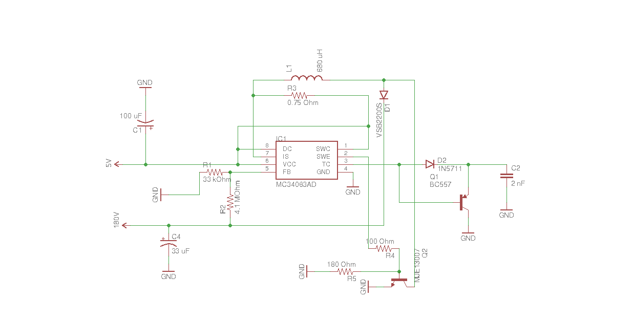
I don’t have a 9-12V power supply, but I have a ton of USB wall warts that output 5V. So I like to power my projects with them when possible. This means I need to learn to make my own power supply! One that will step 5V from a USB supply up to 180V.

Enter the MC34063, a controller for switch mode power supplies. It’s been around for a long time, so it’s easy to find them used in other people’s projects. This allowed me to learn to build my own regulator to step the voltage from one of my USB supplies to power my Nixies!


The Regulator Circuit

Getting 180V from a USB wall wart is, to say the least, difficult. The datasheet for the MC34063 is very helpful, but the example circuits it presents won’t step 5V to 180. The best I could get from the circuit in figure 9 of the datasheet was around 75V.

Part of the problem is that the MC34063 can’t switch fast enough. This can be fixed by using the “ratio extender” circuit described in figure 19 of the application note for the MC34063. Too bad that only got me up to around 85V. And using an external current boost transistor as in figure 10 of the datasheet only pushed it up to 90V.

Luckily, this guy’s website is super helpful. He presents a great design for a high voltage power supply based on an MC34063 and I managed to adapt his circuit for my purposes. See below for the breadboard layout and schematic. The red wire on the right of the board is for Vin and the red wire on the left is the 180V output.

nixie power supply breadboard

breadboard layout for 180V power supply for nixie tubes


nixie power supply schematic

180V power supply for nixie tubes


The Nixie Circuit

The breadboard layout below allows an Arduino to control a single nixie tube using a K155ID1 nixie controller. The K155ID1 takes input from 4 I/O pins on the Arduino. It interprets the high/low signals as a 4 bit binary number. For example, if the signal from the Arduino is LOW, LOW, HIGH, LOW, or 0010 the controller grounds the “2” cathode, which causes it to glow. Be careful when wiring this up because the ordering of the pins on the K155ID1 is not logical. And the way the chip interprets its inputs is also not logical. Check the datasheet.

Notice the red wire leading off to the right of the image. That’s the +180V wire from the power supply. I’m going to skip example code for a single nixie. If you really need code for a single nixie it can be adapted from the code for the multiplexed setup below.

single nixie controller

control circuit for a single nixie


Controlling Multiple Nixies

The way I’ve chosen to control multiple nixie tubes is through multiplexing. This means the cathodes of the nixie tubes are wired in parallel to the same K155ID1 controller chip. The anodes are switched on and off by the Arduino via discrete transistors. The Arduino alternately switches the anodes of each tube on every 5 milliseconds making each tube flash alternately. Even though the tubes are actually flashing, persistence of vision makes them appear to be steadily lit.

It is possible to drive multiple nixie tubes without multiplexing, but multiplexing provides a couple of important advantages. First, without multiplexing, each additional tube requires its own K155ID1 controller IC and 4 additional pins on the Arduino. Multiplexing means we only need 1 controller IC for all of the tubes, and additional tubes only require 1 additional pin.

Second without multiplexing, the current required from the nixie power supply is equal to the current required for a single tube multiplied by the number of tubes. The required current for multiplexed tubes is equal to the current for a single tube. That means the current required from the power supply for multiplexed tubes is much lower. This is good because I really don’t want to push the limits of the power supply I built.

Multiplexing requires a little extra complexity in the code and it makes the tubes appear a little bit dimmer, but I think those costs are worth the benefits.

The breadboard layout below is, admittedly, a hot mess. It somehow looks better on an actual breadboard. It does, however, allow for multiplexed control of multiple nixie tubes. Note that the PNP is an MPSA92 and the NPN is an MPSA42. Note also that the red wire running off to the right of the breadboard is for the 180V input.

multiplexed nixie

breadboard layout for multiplexed nixies


Example Code

The code below displays a count on the two multiplexed nixies in the breadboard layout above. The two tubes count from 00 to 99, incrementing the count every half second. The count resets to 00 once it hits 99.

const uint8_t numTubes = 2;
const uint8_t tubes[numTubes] = {4, 5};
const uint8_t numbers[10][4] = { {0, 0, 0, 0},  // 0
                                 {0, 0, 0, 1},  // 1
                                 {0, 0, 1, 0},  // 2
                                 {0, 0, 1, 1},  // 3
                                 {0, 1, 0, 0},  // 4
                                 {0, 1, 0, 1},  // 5
                                 {0, 1, 1, 0},  // 6
                                 {0, 1, 1, 1},  // 7
                                 {1, 0, 0, 0},  // 8
                                 {1, 0, 0, 1}}; // 9};

uint8_t curTube, curNum;
long tubeSwitchTime, numSwitchTime;
uint8_t digits[numTubes] = {0, 0};

void setup()
{
  for (int i = 0; i < 6; i++)
    pinMode(i, OUTPUT);
  curTube = 0;
  curNum = 0;
  tubeSwitchTime = millis();
  numSwitchTime = millis();
}

void loop()
{
  long curTime = millis();
  if (curTime - numSwitchTime > 500)
  {
    numSwitchTime = curTime;
    curNum++;
    curNum = curNum % (uint8_t)pow(10, numTubes);
    for (int i = 0; i < numTubes; i++) 
    {
      digits[i] = curNum / pow(10, i);
      digits[i] = digits[i] % 10;
    }
  }
  if (curTime - tubeSwitchTime > 5)
  {
    tubeSwitchTime = curTime;
    digitalWrite(tubes[curTube], LOW);
    curTube++;
    curTube = curTube % numTubes;
    for (int i = 0; i < 4; i++)
    {
      digitalWrite(i, numbers[digits[curTube]][i]);
    }
    digitalWrite(tubes[curTube], HIGH);
  }
}


If you did everything right, your nixies should look like this:

2 digit nixie count


Weighted Linear Regression for Wall Following

I’m currently working on a wall-following program for Colin, my mobile robot. True to form, I’ve added an extra complication to the problem: Colin won’t respond directly to his sensor inputs. Instead, he’ll use his sensor inputs to create a simple model of his environment. Then he’ll decide how to move based on this model.

In order to follow a wall, Colin only needs to know the position of the wall relative to himself. To do this Colin will calculate the (x, y) coordinates of each obstacle detected by his rangefinders. Then he’ll fit a line to those points and assume that line represents the wall he’s supposed to be following.

I’ll discuss the actual wall following algorithm in detail in my next post. I’m laying out my method for fitting lines to Colin’s sensor readings in a separate post so I don’t get bogged down in the underlying maths when I’m presenting the wall-following algorithm. If you’re not interested in the maths feel free to skip this post; you can use my line fitting classes without understanding their inner workings. If you want to see what’s going on under the hood, read on.


Interpreting Range Readings

The first thing Colin does is take the range readings from his sonar sensors and convert them into (x, y) points in his local coordinate system. To do this Colin combines his the range readings from his sensors with the orientations of those sensors relative to his heading, which are constant. This turns his range readings into points in a polar coordinate system defined by (r, θ). Then converting these polar points to Cartesian coordinates is pretty easy. Colin calculates the x and y coordinates of each point as follows:

x_{i}=r_{i}cos(\theta_{i})

y_{i}=r_{i}sin(\theta_{i})

In the above two equations, r_{i} is the range reading from sensor i and \theta_{i} is the angle of sensor i relative to Colin’s heading.

My Point data structure does this conversion automatically. Its constructor takes the polar coordinates of the point as arguments and automatically calculates the Cartesian coordinates. It also stores r, as this is used to assign weight to the point later in the program.


Line Fitting

After converting his sensor readings to an array of Cartesian points, Colin fits a line to them. One of the simplest ways to do this is with least-squares linear regression, which works as follows. Assume the following equation describes all of the points:

y_{i}=a+bx_{i}+\epsilon_{i}

Where y_{i} and x_{i} are coordinates of point i, a and b are the slope and intercept of the fitted line, and \epsilon_{i} is the error between the line and point i. Least squares regression determines coefficients a and b such that the sum of squares of the errors, \sum_{i=0}^{n}\epsilon_{i}^{2} is minimized.

In terms of linear algebra, the line equation is represented byAx=B where A is an n by 2 matrix containing the x values of Colin’s points:

A=\begin{bmatrix} 1 & x_{0} \\ 1 & x_{1} \\ 1 & x_{2} \\ ... & ... \\ 1 & x_{n} \\ \end{bmatrix}

B is an n by 1 vector containing the y values of Colin’s points:

B=\begin{bmatrix} y_{0} \\ y_{1} \\ y_{2} \\ ... \\ y_{n} \\ \end{bmatrix}

and x is a 2 by 1 vector containing the y intercept and slope of the fitted line.

x=\begin{bmatrix} a \\ b \\ \end{bmatrix}

Unfortunately, there is usually no x vector that satisfies Ax=B for every entry in the A and B matrices because all of the points will not lie on the same line. What we want, then, is a vector \hat{x} that minimizes the sum of squares of the errors for each entry. The equation for \hat{x} is as follows:

A^{T}A\hat{x}=A^{T}B

This equation can be solved pretty simply by multiplying both sides by the inverse of A^{T}A:

\hat{x}=(A^{T}A)^{-1}A^{T}B

The above equation calculates the slope and y intercept of the line that best fits all of Colin’s sensor readings. That brings us a step closer to our goal!

Also, the math presented above is only a very high-level overview. If you’d like to go more in-depth I’d recommend this very thorough textbook chapter from MIT.


Weighting the Points

You may have noticed a problem with the idea of using simple linear regression to model walls. Most of Colin’s sensors will either detect no obstacle or they will detect a far-away obstacle that is not part of the wall Colin is following. This means that most of the points are not relevant. At most three or four of these points will actually represent a wall.

Very distant points are likely to represent failed readings or obstacles that aren’t relevant to Colin’s decision making. So I decided that points that are more distant from Colin should be less significant and closer points should be more significant. Using this criteria, Colin uses a simple weighting function to assign significance to his points:

w_{i}=\exp(-\frac{d_{i}^{2}}{c})

where w_{i} is the weight assigned to point i, d_{i} is the distance between Colin and point i, and c is a constant. The weighting function’s graph looks like this:

weight-functionThe function assigns a weight of 1 for a distance of 0. Varying the value of c adjusts the distance at which the weight decays to 0.


Weighted Linear Regression

Colin uses the above weighting function to create a weights matrix, W:

W=\begin{bmatrix} w_{0} & 0 & ... & 0 \\ 0 & w_{1} & ... & 0 \\ ... & ... & ... & ... \\ 0 & 0 & ... & w_{n} \\ \end{bmatrix}

As you can see, W is a diagonal matrix of the weights assigned to each point. It fits into the linear regression equation as follows:

A^{T}WA\hat{x}=A^{T}WB

Similar to the unweighted regression, this is solved for \hat{x} by multiplying both sides by the inverse of A^{T}WA:

\hat{x}=(A^{T}WA)^{-1}A^{T}WB

Using the above function Colin calculates the equation of a line fitted to the obstacles that are closest to him and therefore most likely to be relevant to his decision making.

My class, LineFitter, stores an array of Points and automatically fits a line to those points using the above method for weighted linear regression. This makes it very easy to use in my wall following program, which I will present in my next post.


Alternate Methods

A more sophisticated method would incorporate RANSAC to determine which points actually represent the wall and then fit a line to those points, ignoring the others. It would be very interesting to try to implement this method and compare its performance to my simple weighted linear regression. However, I don’t believe Colin would benefit much from using the more sophisticated method in his current configuration.

This is because Colin is working with a very small data set of only 8 points. This means the both my method and RANSAC could easily find spurious relationships in the data. Further, RANSAC is probably overkill; a brute-force search for relationships between Colin’s points would probably be more efficient on such a small data set. Since both are workable and weighted regression is much easier to implement, that’s where I’m starting. This is a good excuse to do further research on RANSAC, though, and I may do a post on that topic in the future.


ATtiny Sonar Controller

HC-SR04 sensor

Remember these guys? HC-SR04 ultrasonic rangefinders. Colin used to have three of them, but I’ve recently been reworking his sensor layout. I’m starting by adding five more sensors for a total of eight. Colin’s Arduino has just barely enough free pins to accommodate eight sensors, but I don’t want to spend all of my available pins on sensors. That would leave me no room to expand. Further, I’m not totally sure eight sonar sensors will be enough. My HC-SR04 sensors have a range of about 15 degrees, so it would take 24 sonar sensors to cover 360 degrees. I don’t know if that will be necessary, but I’d like to have the option.

There are a couple of ways to do this. The simplest would probably be to use a shift register. Shift registers allow you to use three I/O pins to control more than a thousand additional pins, but operating them involves some computing overhead and the Arduino still has to be involved in every sensor reading operation.

The chip for my sonar controller, an ATtiny84

An Atmel ATtiny84

The method I’ve chosen is to use a separate microcontroller, an ATtiny84, to handle the sonar sensors. The Aduino tells the ATtiny that it needs new sensor readings. Then it goes and performs some other computations while the ATtiny pings its sensors. Then, when the new sensor data is ready, the ATtiny sends back the new readings all at once. Using this scheme, the Arduino doesn’t have to spend processor time reading sensors. Instead it can focus on other problems. Also, since it can communicate with the Arduino via I2C, it only requires 2 I/O pins! Here’s what Colin looks like with his new sonar layout.

Colin with his new sonar

Colin with his new sonar ring

As with my earlier post on Raspberry Pi to Arduino communication, there’s several steps to this process. Luckily it’s a lot simpler this time.


The Communication Protocol

The communication protocol is going to be very similar to the one that I outlined for communicating between a Raspberry Pi and an Arduino, only simplified. Basically, the Arduino tells the ATtiny when it needs updated sonar readings. The ATtiny then pings all of its sensors and sends back the readings when it’s done. This is how it works:

  • The Arduino sends a byte to the ATtiny
    • The byte has no meaning, it’s just a flag to signal the ATtiny to ping its sensors
  • The ATtiny pings its sensors
  • The ATtiny sends its readings back to the Arduino as 16 bytes
  • The Arduino assembles the bytes into 8 16-bit ints

One other difference with the Raspberry Pi to Arduino protocol is that we’ll be using I2C instead of serial. If you’re not familiar with I2C I’d suggest reading up on it. Sparkfun has a great tutorial.

That’s really all there is to it! The protocol is simple, but there’s some fiddly details to work out in the code.

Top of page


The Sonar Controller

sonar controller with ATtiny84

My ATtiny84-based sonar controller

My sonar controller basically consists of an ATtiny84, with eight inputs for HC-SR04 ultrasonic rangefinders. If you’re interested in making your own, you can download my eagle files for the schematic, board layout, and the gerber files for fabbing the PCB. The gerbers are formatted for fabrication by OSH Park, which I highly recommend for low-volume jobs.

The controllers each have two sets of inputs for power and I2C communication so multiple controllers can be chained together on the same bus. Note that there are two spots for 4.7 kOhm resistors on each controller. These are pull-ups for the I2C buses. If you’re chaining multiple controllers together, only one of them needs pull-up resistors. The resistor spots on the other controllers can be left empty.

I also designed a laser-cut frame to hold the sonar sensors and controller, as well as some fittings to attach the whole business to Colin. The design is pictured below, and you can download the SVG files to make your own parts here.

Colin's new sonar arrangement

Colin with his new sensor arrangement and fittings

If you’d rather not fab a custom circuit board, you can set it up on a breadboard as shown below. It’s not particularly useful on a breadboard, but it will allow you to experiment with and test it.

breadboard wiring

Breadboard wiring for ATtiny sonar controller

Top of page


The Code!

ATtiny Code

Let’s start out with a couple of preliminaries. First, for I2C communication I’m using the TinyWireS and TinyWireM libraries. We need our ATtiny to perform as both master and slave, but there is no existing library that allows this. Fortunately there’s a way to hack around this problem.

I’m also using the NewPing library. The NewPing library doesn’t work with ATtinies, but there’s a hack for this too. You just need to comment out the functions for Timer2 and Timer4 because the ATtiny does not have these timers.

You can find the complete program for the ATtiny here. If you’re not familiar with how to program ATtinies, I’d suggest going through this very thorough tutorial.

Initiating A Sensor Update

The function below pings the eight sonar sensors and records the ping times in microseconds.

void updatePingTimes(uint8_t bytes)
{
  TinyWireS.receive();
  for (int i = 0; i < NUM_SONAR; i++)
  {
    pingTimes[i] = sonar[i].ping();
  }
  sendTimes();
}

The function above is invoked using an interrupt when the ATtiny receives a byte from the Arduino. The line below is called in the setup() function to tell the ATtiny to generate an interrupt and call the updatePingTimes() function whenever data is received from the Arduino.

TinyWireS.onReceive(updatePingTimes);

Sending Data Back To The Arduino

When the sonar sensors have been updated, the sendTimes() function is called to send the updated ping times back to the Arduino. It is important to note that the ATtiny must be functioning as a slave in order to use the onReceive() function. To send data back to the Arduino, the ATtiny must function as a master. This makes the sendTimes() function a bit more complicated.

void sendTimes()
{
  // clear the I2C registers
  USICR = 0;
  USISR = 0;
  USIDR = 0;

  // start I2C with ATtiny as master
  TinyWireM.begin();

  // transmit ping times to Arduino
  TinyWireM.beginTransmission(MASTER_ADDRESS);
  for (int i = 0; i < NUM_SONAR; i++)
  {
    int thisTime = pingTimes[i];
    if (thisTime == 0) thisTime = (double)MAX_DISTANCE / speedOfSound;
    uint8_t firstByte = thisTime & 0xFF;
    uint8_t secondByte = (thisTime >> 8) & 0xFF;
    TinyWireM.write(firstByte);
    TinyWireM.write(secondByte);
  }
  TinyWireM.endTransmission();

  // clear I2C registers again
  USICR = 0;
  USISR = 0;
  USIDR = 0;

  // put ATtiny back in slave mode
  TinyWireS.begin(OWN_ADDRESS);
}

As I said before, I don’t know of any library that allows an ATtiny to function as both master and slave. Fortunately we can hack our way around this problem by clearing the ATtiny’s I2C registers and restarting communication in master mode. After we’ve transmitted the ping times back to the Arduino we need to clear the I2C registers again and put the ATtiny back in slave mode so it can be ready for the next request from the Arduino. I don’t mind telling you it took me a lot of time with the ATtiny’s datasheet to figure out how to make that work.


Arduino Code

For reference you can find the complete program for the Arduino here. To get things going we need to include the Wire library and put the following two lines in the setup() function:

// begin communication with sonar controller
Wire.begin(OWN_ADDRESS);
Wire.onReceive(updateDistances);

Adding the onReceive() function is particularly important because it allows the Arduino to do other processing tasks while the ATtiny pings its sensors. When the ATtiny sends data it generates an interrupt, the Arduino stops what it’s currently doing and receives the new data, then goes back to whatever it was doing before.

Receiving Data

The updateDistances() function works as follows:

// updates sonar distance measurements when a new reading is available
void updateDistances(int bytes)
{
  for (int i = 0; i < NUM_SONAR; i++)
    readSonar(i);
  distancesRead = true;
}

// reads the distance for a single sonar sensor
// expects to receive values as ints broken into 2 byte pairs,
// least significant byte first
void readSonar(int index)
{
  int firstByte = Wire.read();
  int secondByte = Wire.read();
  sonarDistances[index] = ((double)((secondByte << 8) | firstByte)) * speedOfSound * 0.5;
}

Notice that the sonar distance is multiplied by 0.5 when it’s added to the sonarDistances array. This is because the ATtiny returns the total time of flight for the ultrasonic ping. The ping needs to go from the sensor, to the obstacle, and back. This means multiplying the ping time by the speed of sound would result in twice the distance between the obstacle and the sensor.

Requesting An Update

Fortunately, requesting an update is pretty simple. The Arduino just needs to send a byte, any byte, to the ATtiny to let it know it needs new sensor readings.

// requests a sonar update from the sonar controller at the given address
// by sending a meaningless value via I2C to trigger an update
void requestSonarUpdate(int address)
{
  Wire.beginTransmission(address);
  Wire.write(trig);
  Wire.endTransmission();
}

After this function executes, the Arduino can perform other processing tasks until the ATtiny sends back updated sonar readings.

Top of page


Going Further

There are a number of ways to solve the problem of coordinating large numbers of sonar sensors, and the above method is only one possibility. It takes a long time to update sonar sensors, up to 15 milliseconds for 8 sensors. For an Arduino running at 16 MHz, that’s 240,000 processor cycles. So it’s advantageous to use a method that allows the Arduino to do something else while the sensors are being updated. My method does this, but one could also take the Arduino out of the loop entirely and have the Raspberry Pi talk to the sonar controller directly. It would be interesting to implement this method and compare it to the one presented above.

Top of page

Raspberry Pi to Arduino Communication For Robot Control


Arduino to Raspberry Pi communicationGood news, everyone! I’ve come up with a good way for Colin’s Raspberry Pi to talk to his Arduino. To review, the idea was that the Arduino could handle low-level control functions like speed control, odometry, and sensor reading. This leaves the Raspberry Pi free to handle high-level control like obstacle avoidance, motion planning, and state estimation.

There are a few steps in this process:


Freeing Up the Raspberry Pi’s Serial Port

The first problem we have to deal with is that the Raspbian reserves its serial port for use by a serial console. So the Raspberry Pi’s GPIO serial port is totally useless until you free it up. I’m not going into all the details here, but I found this guide really helpful. The important things to remember are that you need to enable uart in config.txt and disable the serial console. This will allow our program to use the serial port.

Top of page


The Communication Protocol

The communication protocol works like this:

  • The Raspberry Pi sends 2 16-bit ints to the Arduino
    • The first int is the commanded translational velocity
    • The second int is the commanded angular velocity
  • The Arduino sets its speeds accordingly and then updates its sonar sensors
  • After the sensors are updated, the Arduino sends 11 16-bit ints back to the Raspberry Pi
    • The first 8 ints are the distance readings from the 8 sonar sensors
    • The last 3 ints are the Colin’s x and y position and his heading, calculated from odometry

Using this protocol, Colin will run at the commanded speeds until he receives another command. This causes a problem: Colin will continue to run even if the serial communication fails and the Raspberry Pi stops sending commands all together. This means he could run off a cliff and there would be nothing to stop him!

To fix this I have the Raspberry Pi send commands at a regular interval. If, for example, Colin expects to get a new command every quarter second and he doesn’t get a command at the expected time, he will know there’s a communication problem. If Colin detects a communication fault he can respond in a fail-safe manner by stopping.

Communication Formatting

How do we send ints over serial though? Arduino’s Serial.print()  function converts int and float values to strings of chars before sending them. At first this might seem really convenient, but it actually causes more problems than it solves. First, Arduino and C++ don’t have a great function for converting char strings to int or float values. Second, C++ doesn’t automatically convert numerical types to strings before sending them via serial, so you’d need to write your own function for that. Lastly, if we convert numbers to strings, their lengths will be variable. This means we would need to define some way to tell when one value ends and the next begins.

The good news is none of that is necessary! You know why? Every command and sensor packet will be exactly the same length: 2 16-bit ints for commands and 11 16-bit ints for responses. Further, the ints will always come in the same order. So the meaning of each byte is predictable.

The only problem is you can only send individual bytes over serial. But this is easily solved by splitting the ints into their component bytes before sending:

char firstByte = (byte)(value & 0xFF);
char secondByte = (byte)((value >> 8) & 0xFF);

and reassembling them on the other end:

int value = (secondByte << 8) | firstByte;

Top of page


Wiring It Up

Wiring up the Raspberry Pi to the Arduino is pretty simple, but there’s an important catch. The Raspberry Pi uses 3.3 volt logic and the Arduino uses 5 volt logic. So we need to use a level shifter to allow communication between the two devices. If the level shifter gets a 3.3 volt signal on the low side, it sends out a 5 volt signal on the high side. If it gets a 5 volt signal on the high side it sends out a 3.3 volt signal on the low side. Pretty simple, right? Wire it up as shown below:

wiring for serial between an rPi and an Arduino

Wiring for serial between a Raspberry Pi and an Arduino


Top of page


The Code!


Okay, enough talk. Let’s get into the code. I’m going present the code for the Raspberry Pi side first, and follow it up with the Arduino code. The complete code for the Raspberry Pi can be found here and the Arduino code can be found here.

Raspberry Pi Code

Opening the Serial connection

First, we need to open a serial connection with the Arduino. This is handled by the following function, which I adapted from this extremely helpful site. Check out that site if you want details on how all of this works.

void SerialBot::openSerial()
{
	serialFd_ = open("/dev/serial0", O_RDWR);
																						// to allow blocking read
	if (serialFd_ == -1)
	{
		cerr << "Error - unable to open uart" << endl;
		exit(-1);
	}	
	
	struct termios options;
	tcgetattr(serialFd_, &options);
	options.c_cflag = B9600 | CS8 | CLOCAL | CREAD;
	options.c_iflag = IGNPAR;
	options.c_oflag = 0;
	options.c_lflag = 0;
	tcflush(serialFd_, TCIFLUSH);
	tcsetattr(serialFd_, TCSANOW, &options);
}

There is one important difference between my function above and the one it’s adapted from: I dropped the O_NOCTTY and O_NDELAY flags from the open command in line 3. This means my serial connection will be blocking. In other words, when I call the read() function the program execution stops until there is data to read in the serial buffer. In other words, my program will wait for a response from the Arduino before continuing.

Sending Commands

Sending a command works as follows:

int SerialBot::transmit(char* commandPacket)
{
	int result = -1;
	if (serialFd_ != -1) 
	{
		result = write(serialFd_, commandPacket, commandPacketSize);
	}
	return result;
}

And, in case you’re wondering, the function that assembles the commandPacket is below.

void SerialBot::makeCommandPacket(char* commandPacket)
{
	int16_t intAngular = (int)(angular_ * 1000.0);
	commandPacket[0] = (char)(translational_ & 0xFF);
	commandPacket[1] = (char)((translational_ >> 8) & 0xFF);
	commandPacket[2] = (char)(intAngular & 0xFF);
	commandPacket[3] = (char)((intAngular >> 8) & 0xFF);
}

Note that angular_ is a double representing Colin’s commanded angular velocity. The size and representation of doubles is inconsistent, however, so it’s difficult to break them up and reassemble them on a different machine. Int representations are very consistent, however, so I just multiply angular_ by 1000 to save the first three decimal places and cast it to an int. The loss of accuracy is pretty negligible for our purposes.

Receiving Data

The function below is how we receive data from the Arduino. Note that I’ve set the read to time out after 0.25 seconds. The Raspberry Pi expects to get a response from the Arduino after every command is sent. If it doesn’t receive a response before it’s time to send the next command, it throws an error.

int SerialBot::receive(char* sensorPacket)
{
	memset(sensorPacket, '\0', sensorPacketSize_);
	int rxBytes;
	if (serialFd_ != -1)
	{
		// set up blocking read with timeout at .25 seconds
		fd_set set;
		FD_ZERO(&set); // clear the file descriptor set
		FD_SET(serialFd_, &set); // add serial file descriptor to the set
		struct timeval timeout;
		timeout.tv_sec = 0;
		timeout.tv_usec = 250000;
		
		// wait for serial to become available
		int selectResult = select(serialFd_ + 1, &set, NULL, NULL, &timeout);
		if (selectResult < 0)
		{
			cerr << "blocking read failed" << endl;
			return -1;
		}
		else if (selectResult == 0)
		{
			cerr << "read failed: timeout occurred" << endl;
			return 0;
		}
		else
		{
			rxBytes = read(serialFd_, sensorPacket, numSonar_ + numPoseVariables);
		}
	}
	return rxBytes;
}

Once we’ve read data from the Arduino, we need to parse it:

int SerialBot::parseSensorPacket(char* sensorPacket)
{
	int16_t firstByte;
	int16_t secondByte;
	int16_t inValues[numSonar_ + numPoseVariables];
	for (int i = 0; i < numSonar_ + numPoseVariables; i++)
	{
		firstByte = sensorPacket[2 * i];
		secondByte = sensorPacket[(2 * i) + 1];
		inValues[i] = (secondByte << 8) | firstByte;
	}

	for (int i = 0; i < numSonar_; i++)
	{
		distances_[i] = inValues[i];
	}
	
	x_ = inValues[8];
	y_ = inValues[9];
	theta_ = ((double)inValues[10]) / 1000.0;
}

Note again that Colin’s heading, theta_ , is a double. To save some bother in programming, the double value is multiplied by 1000 and casted to an int before it’s sent. So it needs to be casted to a double and divided by 1000 after it’s received.

Putting It All Together

Okay, last thing: we’ll put all of these things together in a communication function that runs every 0.25 seconds in its own thread:

void SerialBot::commThreadFunction()
{
	while (true) 
	{
		char commandPacket[commandPacketSize];
		makeCommandPacket(commandPacket);
		if (transmit(commandPacket) < 1)
			cerr << "command packet transmission failed" << endl;
		char sensorPacket[sensorPacketSize_];
		memset(sensorPacket, '\0', sensorPacketSize_);
		int receiveResult = receive(sensorPacket);
		if (receiveResult < 1)
		{
			cerr << "sensor packet not received" << endl;
		}
		else if (receiveResult < commandPacketSize)
		{
			cerr << "incomplete sensor packet received" << endl;
		}
		else
		{
			parseSensorPacket(sensorPacket);
		}
		usleep(readPeriod_);
	}
}

Top of page


The Arduino Code

Are you still with me? That took a while, but we got one side of it done. So we just have the Arduino code left to deal with.

Receiving

Let’s start with receiving a command from the Raspberry Pi:

void readCommandPacket()
{
  byte buffer[4];
  int result = Serial.readBytes((char*)buffer, 4);

  if (result == 4) // if the correct number of bytes has been received
  {
    int commands[2];
    
    // assemble 16 bit ints from the received bytes in the buffer
    for (int i = 0; i < 2; i++)
    {
      int firstByte = buffer[2 * i];
      int secondByte = buffer[(2 * i) + 1];
      commands[i] = (secondByte << 8) | firstByte;
    }
    translational = commands[0]; 
    angular = (double)commands[1] / 1000.0; // convert received int to double angular velocity
    colin.drive(translational, angular); // set Colin's speeds
    commandReceived = true; // note that a command has been received
    lastCommandTime = millis();
  }
  else if (result > 0)
  {
    Serial.println("incomplete command");
  }
  // else do nothing and try again later
}

Note that I’m using the Serial.readBytes() function rather than the more common Serial.read() function. There’s a couple of reasons for this. First, Serial.read() only reads a char at a time, but we know we need 4 bytes. Serial.readBytes() also blocks the program’s execution until it receives the requested number of bytes. This is perfect, since it means we’ll get a complete packet, instead of just receiving part of one.

Transmitting

The transmit function first puts all the data that needs to be sent into an array, buffer. Then the buffer is sent to the Raspberry Pi using Serial.write() . Note that I’m not using Serial.print() because it automatically converts int values to characters, and we want to send the bytes exactly as-is.

void sendSensorPacket()
{
  colin.getPosition(x, y, theta); // updates Colin's position
  byte buffer[22];
  addDistances(buffer); // adds sonar readings to buffer
  int sendX = (int)x;
  int sendY = (int)y;
  int sendTheta = (int)(theta * 1000.0);
  buffer[16] = (byte)(sendX & 0xFF);
  buffer[17] = (byte)((sendX >> 8) & 0xFF);
  buffer[18] = (byte)(sendY & 0xFF);
  buffer[19] = (byte)((sendY >> 8) & 0xFF);
  buffer[20] = (byte)(sendTheta & 0xFF);
  buffer[21] = (byte)((sendTheta >> 8) & 0xFF);
  Serial.write(buffer, 22);
}

void addDistances(byte* buffer)
{
  for (int i = 0; i < NUM_SONAR; i++)
  {
    buffer[2 * i] = (byte)(sonarDistances[i] & 0xFF);
    buffer[(2 * i) + 1] = (byte)((sonarDistances[i] >> 8) & 0xFF);
  }
}

Bringing It All Together

The loop() function below brings everything together. It checks to see if there is data in the serial buffer and, if so, attempts to interpret it as a command. If it successfully reads a command, it requests an update from the sonar controller. After the Arduino gets updated sensor readings it assembles a response packet and sends it back to the Raspberry Pi.

Lastly, the Arduino checks to see if more than 1 second has passed since the last command was received. If so, it assumes that a communication fault has occurred and it stops Colin.

void loop() 
{ 
  // check if a command packet is available to read
  readCommandPacket();
  
  // request a sensor update if a command has been received
  if (commandReceived)
  {
    commandReceived = false;
    requestSonarUpdate(SONAR_ADDRESS);
  }
  // send sensor packet if sonar has finished updating
  if (distancesRead)
  {
    distancesRead = false; 
    sendSensorPacket();
  }
  currentTime = millis();
  
  // stop colin if a command packet has not been received for 1 second
  if (currentTime - lastCommandTime > 1000)
  {
    Serial.println("command not received for 1 second");
    lastCommandTime = millis();
    colin.drive(0, 0.0);
  }
}

Top of page


Where Do We Go From Here?

Now we have a good way to communicate between Colin’s Raspberry Pi and Arduino. Colin doesn’t have a way to perceive the world around him, however, so that’s our next step. I designed an independent controller to read Colin’s sonar sensors and relay the information to the Arduino via I2C. My next post will cover the finer details of my sonar controller and the associated communication protocol.

After we sort these details out and get the system working like we want, we can get to programming higher level behaviors. For example, I’m currently working on a wall-following program. I’m hoping it will be ready to present in a couple of weeks! Lots of good stuff to come, stay tuned!

Top of page

Colin’s Spooky Brain Transplant!

In the spirit of Halloween (which I realize was nearly a month ago), I’ve done some unholy, Frankenstein-esque modifications to Colin’s brain!

igor_and_abby


Moving the Arduino to the Breadboard

First of all, I’ve been using an Arduino as Colin’s brain but an Arduino is actually pretty bulky, considering its capabilities. So I’ve replaced this:ArduinoDuemilanove

with this:

atmega328

It’s an ATmega328; the same chip the Arduino uses. If you flash it with an Arduino bootloader you can program and use it exactly like you would an Arduino. This page has a great tutorial for programming and using the bare chip on a breadboard. Also, if you’re willing to pay a little extra you can buy a chip that has the bootloader pre-installed. Both SparkFun and Adafruit sell pre-programmed ATmega328s.

To switch from an Arduino to an ATmega328 I just needed to rejigger my power supply a bit and rewire everything for the new pin mapping (good thing I kept detailed notes on my wiring, right?)

Next, Colin’s control libraries are getting pretty big. Right now they take up about 25% of the ATmega’s memory. When all’s said and done, the control libraries should only be a small part of his program’s total size. So we’re going to need some more space before long.

Also, writing and testing code with the Arduino is getting to be kind of a pain. First, you have to upload your program with the Arduino IDE every time you make a change or want to run a new program. This can get pretty cumbersome, especially if you want to make minor tweaks to a program or try different versions of it. Also, there’s no possibility for multi-threading or concurrent execution. So you’re pretty limited in what your programs can do.


Adding Computing Power!

The solution to this could be to use a more powerful single-board computer like a Raspberry Pi. Since a Pi just runs linux, I can run write, edit, and compile programs on the Pi itself. Also, because it has WiFi, I can leave it connected to Colin and control it via SSH. This makes programming much, much easier. However, it has a couple of significant downsides. It only has one PWM pin, so it can’t directly control two motors. Also, it can’t handle hardware interrupts so it can’t really use motor encoders either.

My solution is to keep the ATmega for low-level motor and sensor control while the Raspberry Pi handles the high-level processing. The Pi and the ATmega will communicate over a serial bus. They will use this to relay commands, position updates, sensor readings, and so on.

This means Colin now has two brains! This is what he looks like with his new braaaains!

colin_with_pi_annotated

Note that the Raspberry Pi uses 3.3V logic and all of the other hardware runs at 5V, so I need to use a level shifter to communicate between the Pi and the ATmega. Also, the Raspberry Pi runs on 5V USB power. I already have my voltage regulator supplying 5V for my ATmega, so I simply cut the end off an old micro USB cable and connected the +5V and GND wires to my breadboard’s power rail. The Pi draws a lot of current, around 1.3A under stress, and my voltage regulator can only provide 1.5 to 1.75A. So I might need to upgrade to bigger voltage regulator soon.

I’m also re-configuring Colin’s sonar sensors. I will start out with 8 sensors arranged in a ring, controlled independently by an ATtiny84. Since each sensor has a range of about 15 degrees, 24 total sensors are necessary to completely cover 360 degrees. I’m not sure I’ll need to actually use 24 sensors, but my design will allow me to add additional sensor rings if necessary. I’ll go into detail on these in a later post.

I’ll explain how to coordinate the raspberry pi and the ATmega328 using serial communication in a later post, and I’ll provide an overview of my ATtiny-based sensor controllers shortly thereafter!

Odometry With Arduino

Now that we can control the speed of Colin’s wheels, we can tell how far Colin has moved using odometry. It involves counting the encoder ticks for Colin’s motors and integrating that information over time to determine Colin’s change in position. This method has the distinct advantage that it relies on the actual motion of Colin’s wheels, and thus doesn’t require absolute accuracy from the speed control algorithm. Odometry also provides a good motion model that can be used as part of a larger localization algorithm. As such it’s a good stepping stone toward my goal of making a simultaneous localization and mapping program for Colin!

This tutorial owes a lot to MIT’s primer on odometry and motor control. It does a great job explaining the theory behind odometry.


Theory Basics

The position of a robot in space is referred to as its pose, which is defined by six quantities: its translation in Cartesian coordinates (x, y, and z) and its rotation about those three axes (θx, θy, and θz). Luckily, a differential drive robot like Colin can only translate in two dimensions and rotate in one, so Colin’s pose can be defined by three quantities (x, y, and θz).

Let’s say Colin’s initial pose is (0, 0, 0) at t=t_{0}. How can we determine his change in pose when t=t_{0}+\Delta t where \Delta t is the time interval between pose updates? Because we’re already using encoders to control Colin’s speed, it’s easy to keep track of the distance Colin’s wheels have turned. In fact, my Encoder class already does this with its getDistance() function.

Let’s say d_{left} is the distance turned by the left wheel over \Delta t, and d_{right} is the same quantity for the right wheel. Knowing these two distances can tell us a couple things. If d_{left}=d_{right} then Colin traveled in a straight line. If d_{left}\gt d_{right} he turned to the right and if d_{left}\lt d_{right} he turned left. We can also use d_{left} and d_{right} to calculate Colin’s exact translation and rotation.

To simplify things a bit we’ll assume Colin’s wheel speeds are constant, which adds a negligible amount of error as long as we keep \Delta t small. This assumption means that Colin is always travelling along a circular arc. The length of this arc, d_{center} is given by the average of d_{left} and d_{right}:

d_{center}=\frac{d_{left}+d_{right}}{2}

We’ll say that Colin’s rotation in radians over \Delta t is \phi. Also, let r_{left} be the distance between the center of Colin’s arc of travel and his left wheel and r_{right} be the same distance for the right wheel. This means that d_{left}=\phi r_{left} and d_{right}=\phi r_{right}. Also, r_{left}=r_{right}+d_{wheels} where d_{wheels} is the distance between Colin’s wheels. With a little bit of algebra we can show the following:

\phi=\frac{d_{right}-d_{left}}{{d_{wheels}}}

We can also calculate Colin’s change in his x and y coordinates via the following equations:

x'=x+d_{center}cos(\theta)

y'=y+d_{center}sin(\theta)

Where x' and y' are the new x and y position, respectively. It’s important to note that the above equations are simplified. They assume that Colin’s motion happens in two discrete phases: he rotates in place and then translates along a straight line. This is clearly not true, but as long as \phi is small, the error introduced is negligible. This means that, as with our prior simplification, we need to keep \Delta t small to make this work. I’m not going to go into all the details here, but if you’re interested you can find the full derivation in the MIT odometry tutorial.

So, now that we have worked out the mathematical underpinnings for odometry, we can translate this into code!


Odometry Code

The magic happens in my new DifferentialDrive library. We’ll just go over the odometry portion today, but DifferentialDrive allows the user to control an arbitrary differential drive robot by specifying the robot’s translational and angular velocities and, optionally, the distance the robot should travel. I’ll explain all of that in a later post and include some implementation examples as well!

void DifferentialDrive::updatePosition()
{
   // get the angular distance traveled by each wheel since the last update
   double leftDegrees = _leftWheel->getDistance();
   double rightDegrees = _rightWheel->getDistance();

   // convert the angular distances to linear distances
   double dLeft = leftDegrees / _degreesPerMillimeter;
   double dRight = rightDegrees / _degreesPerMillimeter;

   // calculate the length of the arc traveled by Colin
   double dCenter = (dLeft + dRight) / 2.0;

   // calculate Colin's change in angle
   double phi = (dRight - dLeft) / (double)_wheelDistance;
   // add the change in angle to the previous angle
   _theta += phi;
   // constrain _theta to the range 0 to 2 pi
   if (_theta > 2.0 * pi) _theta -= 2.0 * pi;
   if (_theta < 0.0) _theta += 2.0 * pi;

   // update Colin's x and y coordinates
   _xPosition += dCenter * cos(_theta);
   _yPosition += dCenter * sin(_theta);
}

The above function needs to be called every \Delta t and, to keep the error from our simplifications small \Delta t needs to be small. In my testing I’ve found that doing a position update with the same frequency as the updates for the PID motor controller (every 50ms) results in good accuracy over short distances. However, this update involves a significant amount of extra computation, and doing it 20 times per second might require an excessive amount of processor time if you’re trying to do a lot of other computation at the same time. I’ve found that doing position updates half as often (every 100ms) results in very little loss of accuracy, so it’s entirely possible to balance accuracy and the resources your program has to spare.


Further Work

First of all, we need to integrate the above update function into the larger class that controls Colin’s motion. I’ll demonstrate that in a later post and include some examples that show how to use the class in an Arduino sketch.

Also, odometry can only be used to calculate Colin’s position relative to his starting position. It cannot be used to determine his absolute position in a space unless his starting position is known.

The larger problem is that odometry is inherently inaccurate. Encoder ticks do not translate directly into distance traveled by the wheel because wheels slip, the wheels aren’t perfectly circular, the ground isn’t perfectly flat, encoder ticks might be missed, and the motor gearbox has backlash that isn’t accounted for in our model. This means that Colin’s position calculated from odometry will gradually diverge from his true position. We could use other methods that might be more accurate, such as optical flow and IMUs. However, any sensor we might use suffers from some inherent random error, known as noise, and this error will accumulate over time.

To compensate for this error we can calculate Colin’s probable position by incorporating data from another sensor. This is what I’ll be working on over the next several months. First I’ll develop a program to localize him to a pre-existing (or a priori) map, and then I’ll work on a program that allows him to build his map on the fly.

I should note that software for this purpose is already available as part of the robot operating system (ROS), but I’m not interested in pre-made solutions. My goal here is to develop these solutions myself so we can all learn the intimate details of their operation.

PID Motor Control

Months ago I wrote a post on the use of motor encoders with Arduino and promised to follow up with a post on speed control. In fact at the time I already had a mostly functional speed control class but I decided I had to do some major cleanup on it before presenting here. Then I started school I had no time for Colin or this blog for nine months.

Now, that I’m done with school I’ve had time to write a brand new motor control library! You can find the source code and an example sketch at github.com/1988kramer/motor_control.

In this post I’m going to briefly explain how my motor control program is structured, then give some background on the control theory that went into it, then I’ll explain how the theory is implemented in the actual code.


Program Structure

I structured my program to mirror the hardware as closely as possible so I made two classes, Motor and Encoder, to handle the low level functions of the motor and encoder. The Motor and Encoder classes are used by the SpeedControl class to precisely control the motor’s speed. See the diagram below for a detailed explanation of the the library’s structure.

GDE Error: Error retrieving file - if necessary turn off error checking (404:Not Found)

You’ll notice two classes in the diagram above that use the functionality of SpeedControl: PositionControl and DifferentialDrive. PositionControl uses an instance of SpeedControl to provide position control functions and DifferentialDrive uses two instances of PositionControl to provide high level control for a differential drive robot like Colin.

I’m just going to be discussing SpeedControl class today, but you can expect a post on PositionControl and DifferentialDrive in the next few weeks.


Control Loop Basics

In my earlier post on motor control I explained that simply using analogWrite does not actually set the speed of a motor. It only sets the voltage to the motor. Varying loads will cause a motor to run at different speeds with the same input voltage. How do we get a motor to run at a specific speed? This sounds like a job for a closed-loop controller!

In a closed-loop controller, we tell the controller how fast we want the motor to run. We call this the set point. The controller then measures the actual speed of the motor and calculates the difference between the actual speed and the set point. This is the error. The controller then adjusts the voltage to the motor to reduce the error.

Proportional Control

This sounds simple enough, but how much should the controller adjust for a given error? One could make the adjustment directly proportional to the error, i.e. large errors get large adjustments and small errors get small adjustments. The adjustment would be defined as

A(t)=K_{{p}}e(t)

where A(t) is the adjustment, e(t) is the error, and K_{p} is a constant referred to as the gain. This is a decent solution but it has some problems. If K_{p} is large the controller will be quick to respond to disturbances but it will tend to over-correct (known as overshooting). If K_{p} is very large the motor speed will oscillate around the set point and never stabilize. If K_{p} is small enough to avoid overshooting, however, the controller will respond very slowly to disturbances.

Integral and Derivative Terms

To compensate for this we can add a couple more terms to the adjustment equation. A term proportional to both the error and duration of the error, called the integral term, will correct for persistent small errors that won’t be corrected by the proportional term. It will also make the controller faster to reach the set point. However, if the integral term is too large it will cause overshoot and oscillation. The integral term is defined as

I_{out}=K_{i}\int_{0}^{t}e(\tau)d\tau

Lastly, the derivative (slope) of the error over time can be used to predict the system’s future behavior. For instance, a large derivative indicates the next error will likely be far away from the last whereas a small derivative indicates the next error will likely be close to the last. A term calculated from the derivative of past errors helps to minimize overshoot and improve the stability of the controller. The derivative term is defined as

D_{out}=K_{d}\frac{de(t)}{dt}

PID Adjustment Equation

So our final adjustment is the sum of the proportional, integral, and derivative terms:

A(t)=P_{out}+I_{out}+D_{out}=K_{p}e(t)+K_{i}\int_{0}^{t}e(\tau)d\tau+K_{d}\frac{de(t)}{dt}

Every time the controller adjusts the voltage output to the motor it must find the current speed of the motor, calculate the error between the current speed and the set point, then use the above equation to determine how much the output voltage to the motor should be adjusted to compensate for the error. In Colin’s case this is done 20 times per second.


The Code

Because posting my motor control code in its entirety would take far too much space and most of it isn’t very interesting anyway, I’m just going to post and explain the update function. It calculates the required adjustment to the PWM output to the Motor to maintain consistent speed.

My code draws heavily on Brett Beagregard’s PID library. I would encourage you to check out his blog for a more in-depth explanation of PID control. Thanks for your work, Brett!

// adjusts motor's PWM level to correct for any error between the
// set point and the actual speed of the motor's output shaft
// MUST be called regularly on the same deltaT used to calculate
// motor speed in the Encoder object
void SpeedControl::adjustPWM()
{
	int speed = _encoder->getSpeed(); // motor control returns vector speed
	if (speed < 0) speed *= -1;  // convert speed to scalar
	int error = _setPoint - speed;  // calculate error
	_iTerm += (_kI * (double)error); // calculate integral term
	double dInput = speed - _lastSpeed; // calculate derivative
	int adjustment = (_kP * (double)error) + _iTerm - (_kD * dInput);
	_pwm += adjustment;
	constrainPWM(); // limit _pwm to the range 0-255
	_motor->setPWM(_pwm);
	_lastSpeed = speed;
}

The code above basically performs the calculation discussed in the preceding section. In line 7 it fetches the current speed of the motor and calculates the error in line 9. It then calculates the proportional, integral, and derivative terms and uses them to calculate the adjustment in lines 10 through 12.

Derivative Kick

There is one deviation from the equations presented in the previous section: in lines 11 and 12 we’re using the speed, not the error to calculate the derivative term. Also, we’re subtracting it from the adjustment. What gives?

Basically, when the user changes the set point there is an instantaneous change in the error e(t). This means the derivative of the error \frac{de(t)}{dt} is infinite at this point. So in theory the derivative term becomes infinite whenever the set point changes, a phenomenon called derivative kick. Because the code above calculates the approximate numerical derivative the phenomenon is not as pronounced, but it should still be addressed. Making the change above corrects for derivative kick. See Brett’s blog for a more in-depth explanation.


Example Sketch

So how do we actually implement this to control a motor? You could spend weeks or possibly months of your free time developing a full speed control program, or you could try using the one that I spent weeks of my free time on! The example sketch below demonstrates the use of my SpeedControl class, available on github.

#include <TimerOne.h>
#include <PositionControl.h>

const int dir1 = 9, dir 2 = 8, pwm = 6;
const int encoderA = 3, encoderB = 5;
const int deltaT = 50000;
const int encoderTicksPerRev = 309;
const double kP = 0.025, kI = 0.0008, kD = 0.0005;

Motor rhMotor(dir1, dir2, pwm);
Encoder rhEncoder(encoderA, encoderB, deltaT, encoderTicksPerRev);
SpeedControl rhSpeedControl(&rhMotor, &rhEncoder);

  
void setup() {
  Serial.begin(9600);
  Timer1.initialize(deltaT);
  Timer1.attachInterrupt(adjustPWM);
  attachInterrupt(1, readRHEncoder, CHANGE);
  rhSpeedControl.setGains(kP, kI, kD);
}

void loop() {
  
  rhSpeedControl.setSpeed(180);
  delay(5000);
  rhSpeedControl.setSpeed(0);
  Serial.println(rhSpeedControl.getDistance());
  delay(2000);
}

void readRHEncoder()
{
  rhEncoder.updateCount();
}

void adjustPWM()
{
  rhSpeedControl.adjustPWM();
}

Implementation Notes

A couple of notes on note on the sketch above:

First, the PID gains, kP, kI, and kD used in the example sketch work well for Colin but will need to be tuned for your robot. PID tuning is something of a black art; I haven’t been able to find much info on it online, anyway. The method presented on this wikipedia page worked fairly well for me though.

Second, the SpeedControl.adjustPWM() function must be called every deltaT microseconds using a timer interrupt. See this Arduino playground page for more info on timer interrupts. The deltaT value needs to be tuned just like the PID gains. A deltaT value that’s too large will result in the controller not adjusting frequently enough to accurately control the motor’s speed. A value that’s too small, will limit the accuracy of the speed measurement because fewer encoder ticks can elapse in a smaller amount of time. The maximum accuracy for a given deltaT, by the way, is

Accuracy=\frac{D}{\Delta t}

Where D is the number of degrees per encoder tick. I found a deltaT of 50 milliseconds works well for Colin, but you should play around with it for yourself.

That’s all I have for now! Stay tuned for a post on my PositionControl and DifferentialDrive classes in the next few weeks!

I’m Learning Multithreading!

Since this quarter started I’ve been doing a weekly interview practice session with friends from school. Last week we spent most of our hour on this:

Rotate Matrix: Given an image represented by an NxN matrix, where each pixel in the image is 4 bytes, write a method to rotate the image by 90 degrees. Can you do this in place?

For those interested, it’s exercise 1.7 in the sixth edition of Cracking the Coding Interview by Gayle Laakmann McDowell. It’s a great interview prep book that’s been really helpful since I started job hunting. I had a lot of fun with this one so I’d like to do a short write up on our thought process.


Row-to-Column Method

The obvious thing to do here is create a new NxN square matrix and transpose the rows of the old matrix into the columns of the new matrix as in the graphic below:

MatrixRotateRtC

The above method takes O(n) time and O(n) space where n is the number of entries in the matrix. Coding this up should be pretty simple so I’m going to skip ahead to the thing I’m actually interested in: the in-place method.


In-Place Method

We can’t get below O(n) time to rotate a matrix since every entry must be moved and there are n entries. However, it is possible to cut the space usage down from O(n) to O(1) by doing the rotation in place. See the graphic below for an illustration of the method:

MatrixRotateIP

How do we implement this in code? It’s a little difficult but the key insight is that it’s possible to find the destination index for any given entry in the matrix from its starting index. In general terms the destination index can be found using this relation

Destination for { i, j } = { j, n – i }

where n is the last index in the matrix. The really cool thing about this is that it works for any starting index. The graphic above only shows a rotation of the outer layer of the matrix but the above method works for any index in any size of square matrix.

The code I post on this blog has been getting longer and longer lately, so I’m only going to post the relevant functions on the site. If you want to see the whole program you can find it on my gitHub repo.

The program is called matrixRotate.cpp. It takes a .txt file containing the matrix to rotate as a command line argument. The text file should have one int  representing the size of the matrix on the first line. Each successive line should have a space delimited string of ints representing each row of the matrix. It prints the rotated matrix to the console.

The function below will take care of a single step in the matrix rotation. After the function completes 4 matrix entries are moved.

// accepts three ints, the starting row and column indices
// and the highest index in the matrix, NOT the size
// rotates 4 matrix entries by 90 degrees counterclockwise
void rotateLeftHelper(int row, int column, int n) 
{
  int temp = matrix[row][column];
  for (int i = 0; i < 3; i++) 
  {
    int nextRow = column;
    int nextColumn = n - row;
    matrix[row][column] = matrix[nextRow][nextColumn];
    row = nextRow;
    column = nextColumn;
  }
  matrix[row][column] = temp;
}

To rotate the whole matrix we need to run the above function on every entry in the first row from { 1, 1 } to { 1, n-1 }. Then every entry in the second row from { 2, 2 } to { 2, n-1 }. This needs to be repeated until we get to the starting index: { n/2, n/2 }. The function below will do this for us:

// accepts an int, the matrix size
// rotates the matrix by 90 degrees counterclockwise
void rotateLeft(int n) 
{
  int level = n - 1; // switch n from matrix size to highest index
  for (int i = 0; i < n/2; i++) 
  {
    for (int j = i; j < level; j++) 
    {
      rotateLeftHelper(i, j, n - 1);
    }
    level--;
  }
}

So when they work in concert, the above functions will rotate a matrix by 90 degrees counterclockwise and it’ll do it in place. That’s pretty cool, right? If you’ll recall though, the problem from Cracking the Coding Interview says the matrix represents an image. If it’s a raw image from a run-of-the-mill camera it will have 20 million entries. Doing each rotation in series will tie up the CPU for a long time. Fortunately, using the above  rotateLeftHelper() function, one instance of the function doesn’t affect the others. They never operate on the same part of the matrix! Do you know what that means? They can run in parallel and asynchronously!


Multi-Threaded Version

Really all we need to do here is create a new thread for every call to the rotateLeftHelper() function instead of running them in series. Cool, right?

The function below implements the in-place matrix rotation method using pthreads. See matrixRotate.cpp on my gitHub repo to see the whole program.

// accepts a pointer to a threadParams struct containing three ints, 
// the starting row and column indices
// and the highest index in the matrix, NOT the size
void* rotateLeftHelper(void* start) 
{
  threadParams* startState = (threadParams*) start;
  int row = startState->row;
  int column = startState->column;
  // cout << "starting thread on {" << row <<  ", " << column << "}" << endl;
  int n = startState->n;
  int temp = matrix[row][column];
  for (int i = 0; i < 3; i++) 
  {
    int nextRow = column;
    int nextColumn = n - row;
    matrix[row][column] = matrix[nextRow][nextColumn];
    row = nextRow;
    column = nextColumn;
  }
  matrix[row][column] = temp;
}

// accepts an int, the matrix size
// rotates a matrix by 90 degrees counterclockwise
void rotateLeft(int n) 
{
  int level = n - 1; // switch n from matrix size to highest index
  // calculate number of threads
  int numThreads = 0;
  for (int i = level; i >= 1; i -= 2) {
    numThreads += i;
  }
  pthread_t *threads;
  threadParams *parameters;
  threads = new pthread_t[numThreads];
  parameters = new threadParams[numThreads];
  int curThread = 0;
  for (int i = 0; i < n/2; i++) 
  {
    for (int j = i; j < level; j++) 
    {
      parameters[curThread].row = i;
      parameters[curThread].column = j;
      parameters[curThread].n = n - 1;
      pthread_create(&threads[curThread], NULL, 
		     &rotateLeftHelper, (void*) &parameters[curThread]);
      curThread++;
    }
    level--;
  }
  // join all threads
  for (int i = 0; i < numThreads; i++) 
  {
    pthread_join(threads[i], NULL);
  }
  delete[] threads;
  delete[] parameters;
}

Further Improvements

So the above code will make use of parallel processing to speed up the matrix rotation. However, creating and destroying a thread for each instance of the rotateLeftHelper() function involves an unnecessary amount of overhead. We could avoid that overhead by using a thread pool.

Also, we’re still running the threads on the CPU. In the best case scenario the CPU has 8 cores, so we’ll be getting a speedup factor of much less than 8. That’s good but not great. Also, we’re tying up the CPU to do a lot of extremely simple tasks. It would be better if we had a much larger number of much worse processors to do this task. Does that sound familiar? It’s called a graphics card and it’s what image processing programs on computers actually use to do tasks like this.

I think the best thing I could do for this program would be to figure out how to create threads that run on my graphics card using openGL.

That’s all for now though! Feel free to email me with questions.